Measures are with us since the Excel 2010, yet I’ve seen only a few people using them while doing analysis or data manipulation in any way.
To use Measures in Excel 2010, you first needed to install PowerPivot add-in, since it is not a part of the application itself.
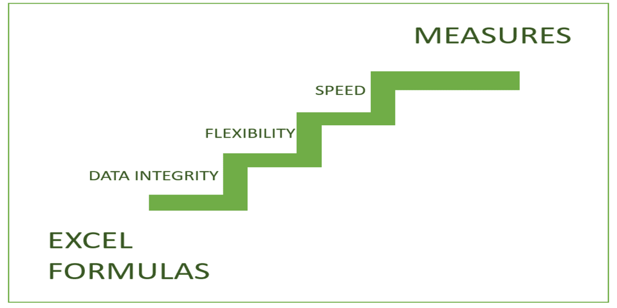
Formulas – The old way
When doing any kind of modeling, colleagues would rely on Excel formulas created across the whole workbook, connected with VLOOKUP od INDEX/MATCH functions. If they were more advanced Excel users, they would also use SUMPRODUCT and OFFSET/INDIRECT to create somewhat dynamic final results.
When created, these models were all performing as expected, but as time passed they all showed flaws.
There were several problems with models created using Excel formulas. I will mention just a few of them:
- Flexibility – No matter how smart and “dynamic” your formulas are, they are still just “formulas” written in cells. You cannot tell formulas in cells “B1:B1000” to transpose and become formulas in cells “B1:ZZ1”, yet to still show expected results. Even if you create dynamic formulas using INDIRECT combined with INDEX/MATCH, they will still fall short if someone wishes to change the dimensions in which they do analysis (for example switch from figures by Brands to figures by Country). Now you could do even that with a help of programming in VBA, but how many people in a regular company possess those skills?
- If you’ve read the above paragraph carefully, you will see that these are the features that made PivotTables such an important part of Excel. The imperfection of PivotTable is that it can do these kinds of data pivoting only with basic functions (like SUM, AVERAGE, COUNT, MIN, MAX). It possesses no advanced formula creation possibilities
- Data integrity – I’m sure that this also happened to you more than once. You create an excellent model based on Formulas then share it with your colleagues to give their input to the provided places in a file (for example cost estimate for each product). Not a five minutes later your excellent model is broken. Why? Some of the colleagues used Cut/Paste numbers which resulted in #REF error across the whole Workbook. You have to find these #REF errors, maybe even resend your file, spending another day of work and running late with other tasks.
- Formulas accuracy – All kinds of user interferences, like inserting/deleting rows, different cells formatting, merging, sorting etc. can break advanced Formulas and most of the time you won’t even notice before it’s too late.
- Formulas usability – Excel formulas are not reusable in other parts of your workbook – for example, you create an awesome formula based on 6 different parameters. Now you want to apply that same formula in the following sheet, but on that sheet, parameters are not in the exact place they have to be. Now you have 2 options: either adjust the formula to new parameter places or adjust parameters to right places before applying a formula. Both of these actions are time-consuming and error-prone and should be avoided if possible.
Issues mentioned above result in redundant work, slower execution speed, lower data flexibility and a high percentage of errors. Most of these errors can get through unnoticed until someone makes a wrong decision based on them, irretrievably damaging company business. The last one does not happen often, but you should do what is in your power to eliminate above problems before it’s too late. And this is where Measures come really handy!
Why Measures
In simple terms, Measures are advanced formulas for the PivotTable. So now instead of just SUM, AVERAGE, COUNT, MIN, MAX you can use any formula you imagine in a PivotTable (ok, this kind of a table is not called PivotTable but PowerPivot, but they practically have the same user interface). To write Measures in PowerPivot, you need a small lecture about the DAX formula language and you are set to go. Now you can write amazing formulas inside PowerPivot, having all the PivotTable pivoting features working impeccably.
To create measures, you first need to add data to Excel data model. The adding part is similar to inserting a PivotTable. You select a range that you wish to work on, go to Insert PivotTable -> When you are prompted with a form asking you where to insert a PivotTable, make sure you mark “Add this data to Data Model” checkbox.
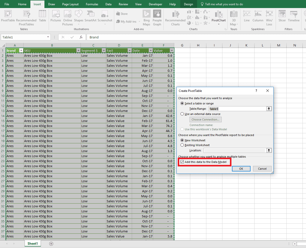
When selecting data for PivotTable/PowerPivot, I would strongly advise you to store all data inside an Excel table through Insert=>Table feature! That way when you add new data to the table, your PowerPivot will automatically include new rows. In case you need to do some data cleanup or data rearranging before importing it into PowerPivot, you can make that changes inside a PowerQuery (another great tool available in Excel 2010 and later versions)!
Imagine that you will receive the same structure of data every month and you need to create a dynamic analysis each time new data arrives. With each month there are new requests coming from management which you need to incorporate into your already existing analysis. Also, your analysis has to be extremely flexible to handle any ad hoc request coming from your superior. With formulas and regular Excel PivotTables, this would be a daunting job full of repetitive work and chances of errors would grow exponentially as the new elements were to be added to your analysis.
How about trying to solve all these problems with PowerPivot Measures?
PowerPivot Measures to the rescue!
With Measures, you can create even more powerful data models/analysis, but without the shortcomings of the Excel formulas. Since every measure resides inside a PowerPivot, they are not cell dependent, meaning all those errors mentioned at the start of the article (Cut/Paste, Inserting/Deleting rows, cell formatting etc.) are eliminated at the very start.
Next, with Measures, you keep all the original PivotTable pivoting capabilities but with much stronger formulas than a regular PivotTable ones.
There are many more advantages of using Measures like the possibility to use data from different sources (linked through relationships), considerably faster execution speed etc., but they are out of the scope of this article.
Ok now let’s try and test those two hypotheses.
Based on the data in the first picture, imagine that we need to create Price per Unit Measure. The simple formula for that is Sales Value / Sales Volume. Our management wants to observe this measure in different situations. Sometimes they want to look at the Manufacturer or Brand level, other times based on segmentation. Also, sometimes they want to see a trend, and other times they want to see long-term development (year on year). You cannot create such a flexible structure using solely Excel formulas and PivotTables (you can but it will take you significantly more time and if would not be cost/time acceptable). This task with Measures? A piece of cake.
After you selected a table and imported it into a data model, you will notice the blank PivotTable with fields shown on the right side of the Worksheet.
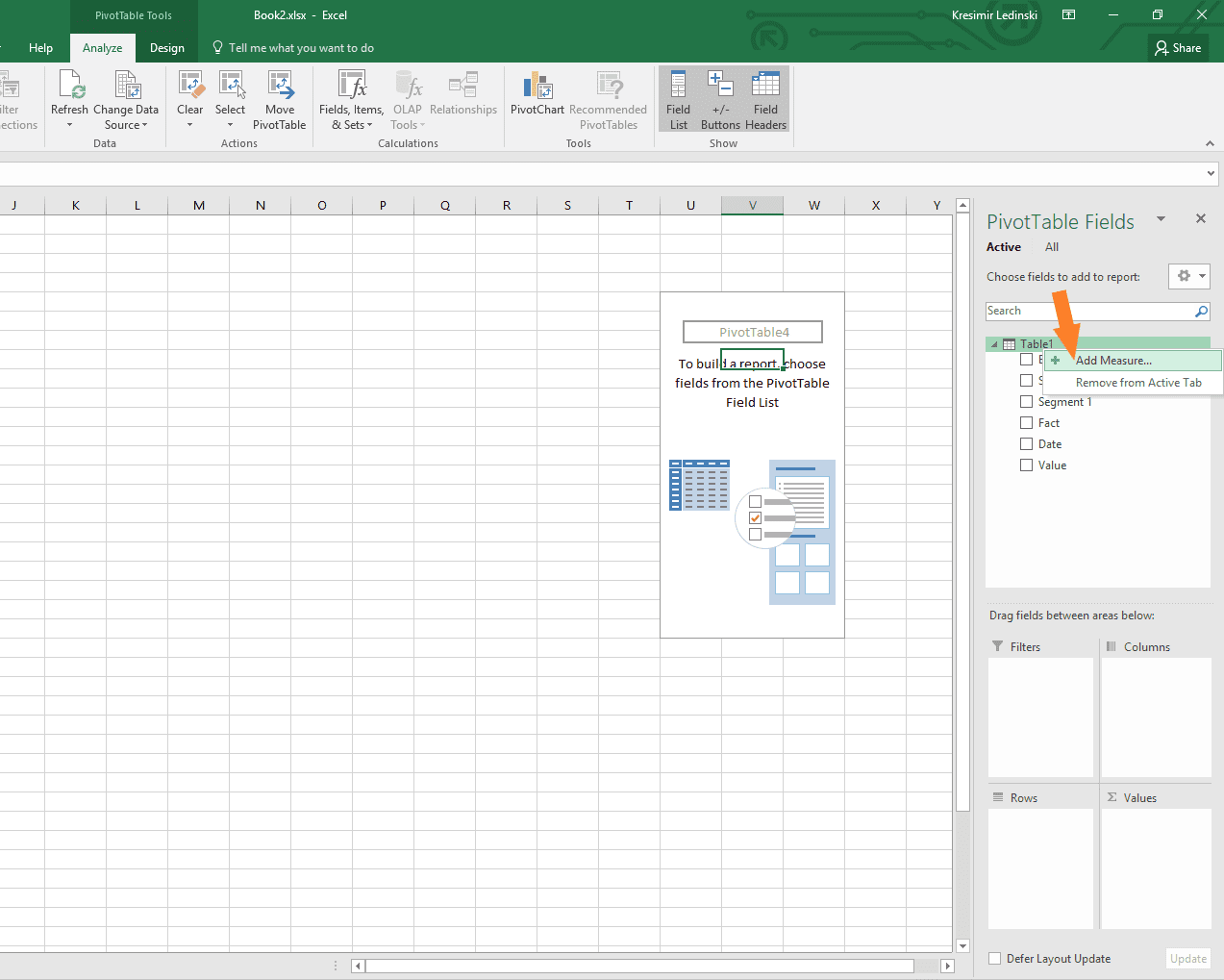
You insert a new measure by going to the table name inside PivotTable fields -> Right click on table name -> Add Measure
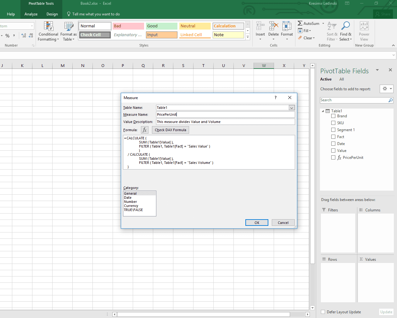
A new form will show up in which you will be able to write the name of the Measure, short description of it, DAX formula, and formatting which will be applied to that Measure. Since in our data table we have both Value and Volume in the same column, we need to filter Sales Value from the column, then divide it by the filtered Sales Volume from the same column. DAX formula for that would be as follows.
=CALCULATE (
SUM ( Table1[Value] ),
FILTER ( Table1, Table1[Fact] = “Sales Value” )
)
/ CALCULATE (
SUM ( Table1[Value] ),
FILTER ( Table1, Table1[Fact] = “Sales Volume” )
)
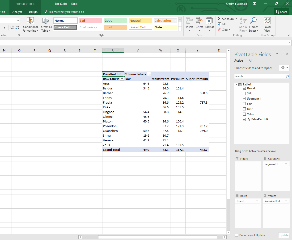
Once you created a Measure, you can apply it to the PivotTable, and it will calculate the correct values no matter how you choose to show your data. For instance, to see how each Brand behaves at each price segment, just drag Segment 1 to the columns, Brand to the rows and newly created Measure to Values field.
PricePerUnit development by Segments for each period is also just 2 clicks away.
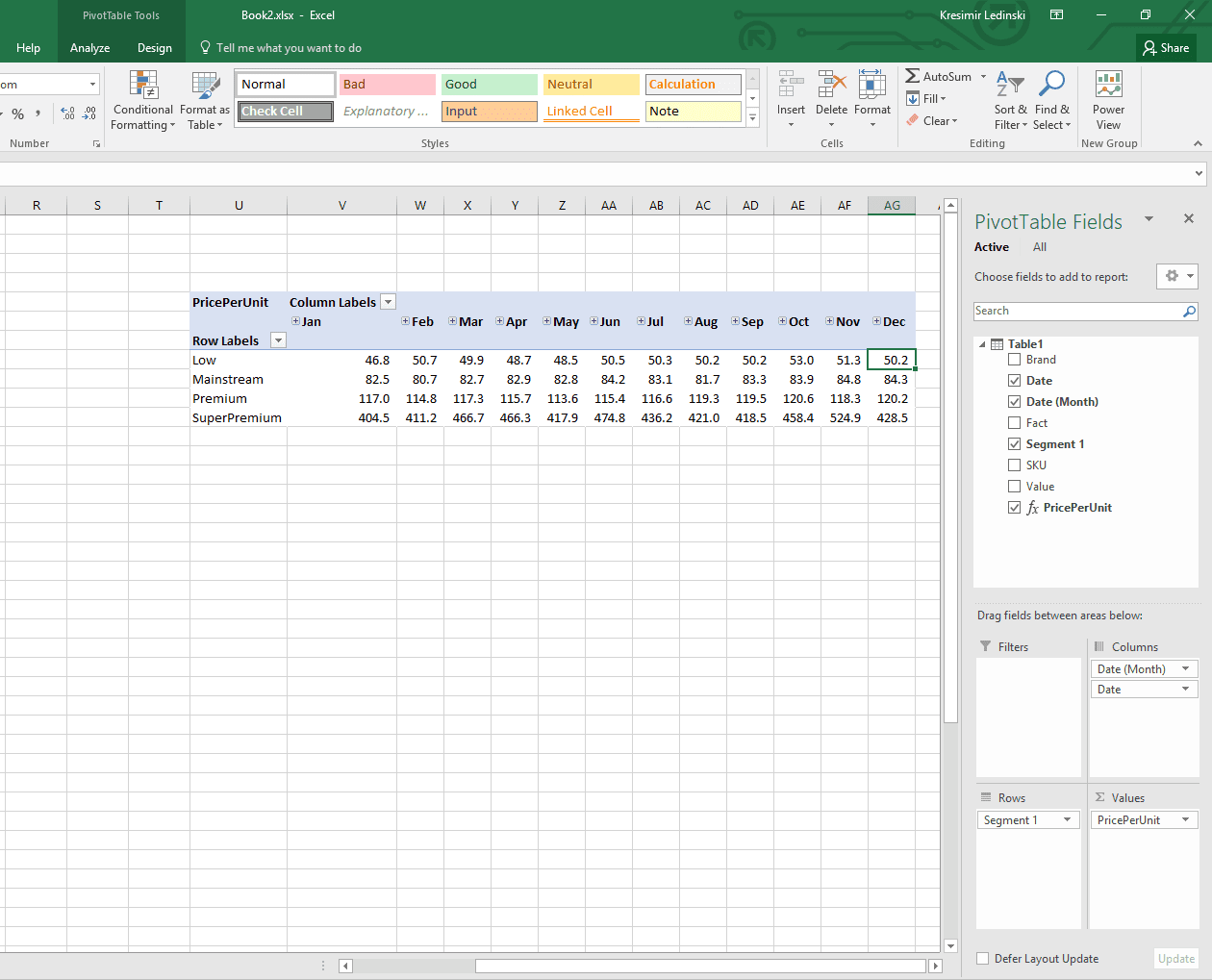
Just imagine how simpler and faster you can create and adjust your analysis combining Measures. Each Measure is portable and can be used in any part of your report/analysis. You can even create Measures based on other Measures! Now combine that with new data modeling capabilities of Excel and Relations, It’s just insane!
Wrap Up
Measures come to the rescue where regular Excel Formulas and PivotTable show their flaws. With Measures, you get all the functionality of the Excel formulas packed with stronger calculation speed, much more flexibility and high data integrity.
For anyone who considers himself a data analyst and does most of his work in Excel, Measures are a must.
Hope you enjoyed reading the article! If you have any questions, please comment below, and if you liked this article, don’t forget to Share/Like!


