Excel Analytics Course
The most important elements of Excel every analyst should understand and use!
Excel Analytics Course
Quiz Summary
0 of 105 questions completed
Questions:
Information
You have already completed the quiz before. Hence you can not start it again.
Quiz is loading…
You must sign in or sign up to start the quiz.
You must first complete the following:
Results
Results
0 of 105 questions answered correctly
Your time:
Time has elapsed
You have reached 0 of 0 point(s), (0)
Earned Point(s): 0 of 0, (0)
0 Essay(s) Pending (Possible Point(s): 0)
| Average score |
|
| Your score |
|
Categories
- Dynamic Array Formulas 0%
- Excel Conditions 0%
- Excel data entry 0%
- Excel Formulas 0%
- Excel Tables 0%
- Merging Sources (VLOOKUP, XLOOKUP, INDEX, etc.) 0%
- PivotCharts 0%
- PivotTables 0%
- PowerPivot basics 0%
- PowerQuery basics 0%
- 1
- 2
- 3
- 4
- 5
- 6
- 7
- 8
- 9
- 10
- 11
- 12
- 13
- 14
- 15
- 16
- 17
- 18
- 19
- 20
- 21
- 22
- 23
- 24
- 25
- 26
- 27
- 28
- 29
- 30
- 31
- 32
- 33
- 34
- 35
- 36
- 37
- 38
- 39
- 40
- 41
- 42
- 43
- 44
- 45
- 46
- 47
- 48
- 49
- 50
- 51
- 52
- 53
- 54
- 55
- 56
- 57
- 58
- 59
- 60
- 61
- 62
- 63
- 64
- 65
- 66
- 67
- 68
- 69
- 70
- 71
- 72
- 73
- 74
- 75
- 76
- 77
- 78
- 79
- 80
- 81
- 82
- 83
- 84
- 85
- 86
- 87
- 88
- 89
- 90
- 91
- 92
- 93
- 94
- 95
- 96
- 97
- 98
- 99
- 100
- 101
- 102
- 103
- 104
- 105
- Current
- Review
- Answered
- Correct
- Incorrect
-
Question 1 of 105
1. Question
Category: PowerQuery basicsWhich of the following best describes the PowerQuery tool?
CorrectIncorrect -
Question 2 of 105
2. Question
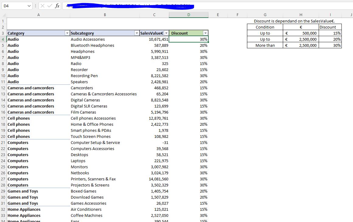
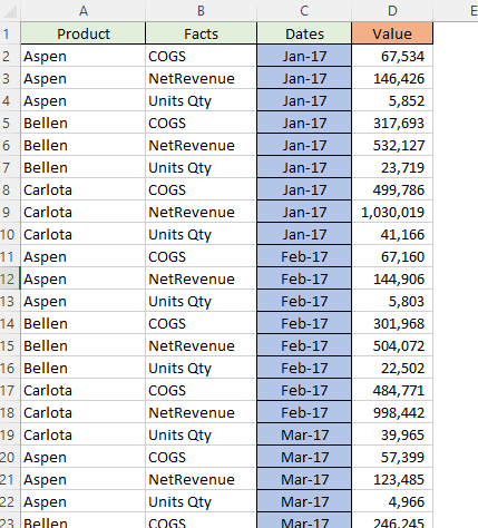
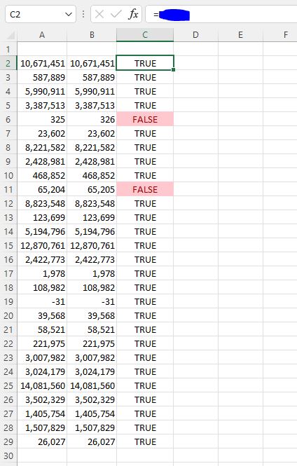
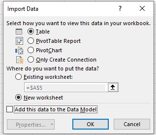
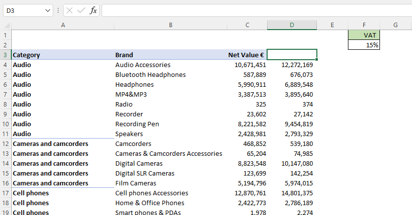
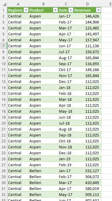
Category: Excel ConditionsDownload the following Excel workbook and use it to answer the question.

We want to add a formula in the D column using the following condition: if the category is Cameras and camcorders (cell J3 value), and SalesValue€ is above 5.000.000€ (cell I3 value), then 15% discount is applied (cell K3 value).
Which formula should be entered into cell D4? The formula should show the correct result when copied across the whole D column.
CorrectIncorrect -
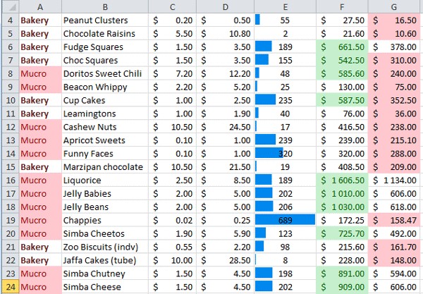
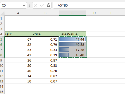
Question 3 of 105
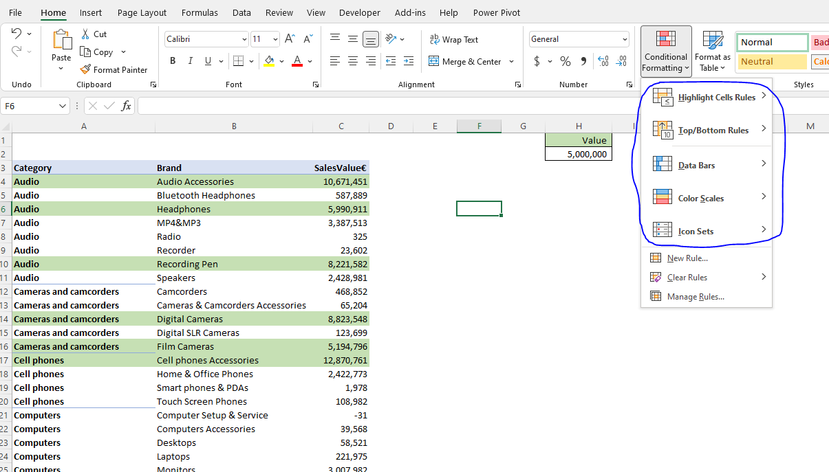
3. Question
Category: Excel ConditionsWe want to apply conditional formatting in the table below. The condition is that for any value greater than 5.000.000 (cell H2 value), the whole row of the table needs to turn green.
Sort in the correct order actions you need to use to add this type of conditional formatting to your data range.
-
Apply formatting rule
-
enter manual format rule (=$C4>$H$2) and define formatting options
-
Select "Use a formula to determine which cells to format" option
-
Go to Conditional formatting Tab
-
Select "New Rule option…"
-
Select the range A4:C1000
CorrectIncorrect -
-
Question 4 of 105
4. Question
Category: Merging Sources (VLOOKUP, XLOOKUP, INDEX, etc.)Which of the following functions can you use to return multiple matching rows when performing lookup operations?
CorrectIncorrect -
Question 5 of 105
5. Question
Category: PowerQuery basicsWhat are the main features of PowerQuery?
CorrectIncorrect -
Question 6 of 105
6. Question
Category: Dynamic Array FormulasWhat are the advantages of using modern Array formulas?
CorrectIncorrect -
Question 7 of 105
7. Question
Category: Excel ConditionsStudy the screenshot below. Several Conditional Formatting rules have been applied to this worksheet.
How can you ascertain which rules have been applied and where?
CorrectIncorrect -
Question 8 of 105
8. Question
Category: Excel ConditionsDownload the following Excel workbook and use it to answer the question.
We want to add condition in D column using conditions set in table in range G3:I4.
Which formula should be entered into cell D4? The formula should show the correct result when copied across the whole D column. Use table and absolute references where necessary.
CorrectIncorrect -
Question 9 of 105
9. Question
Category: PivotTablesWhich PivotTable feature do we need to use to calculate the average of Unit price?
CorrectIncorrect -
Question 10 of 105
10. Question
Category: Dynamic Array FormulasCan you use modern array functions as a source for data validation list, like in a picture below?
CorrectIncorrect -
Question 11 of 105
11. Question
Category: Merging Sources (VLOOKUP, XLOOKUP, INDEX, etc.)Select all advantages when using XLOOKUP function compared to VLOOKUP:
CorrectIncorrect -
Question 12 of 105
12. Question
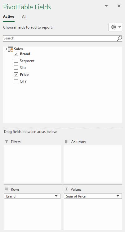
Category: PivotTablesIs this an optimal data source structure for importing in a PivotTable?
CorrectIncorrect -
Question 13 of 105
13. Question
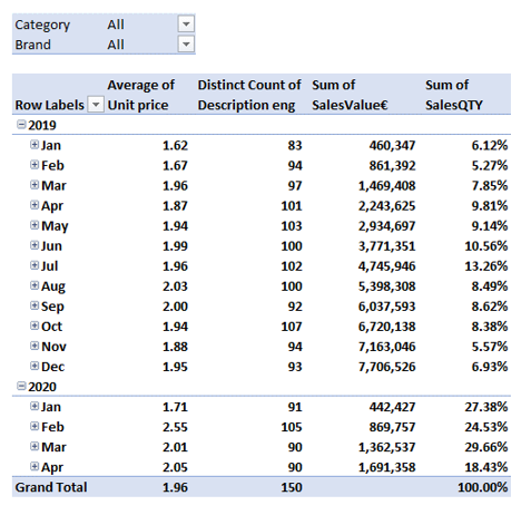
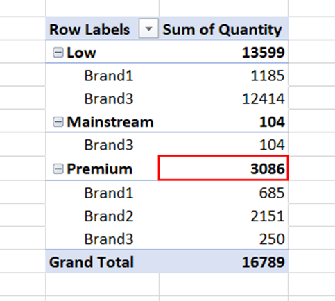
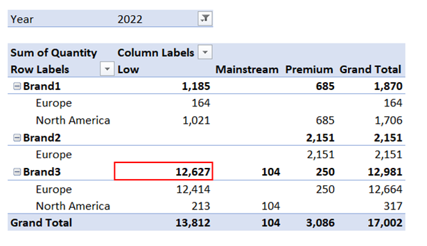
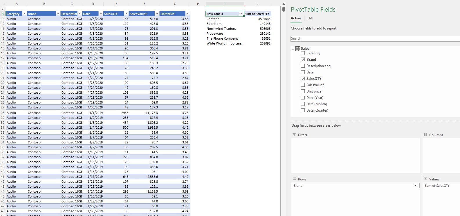
Category: PivotTablesWhich PivotTable feature do we need to use to calculate the % share of SalesQTY in a selected Year (the last column in the visual below)?
CorrectIncorrect -
Question 14 of 105
14. Question
Category: Dynamic Array FormulasHow can we show a result of an array function in a data validation list?
CorrectIncorrect -
Question 15 of 105
15. Question
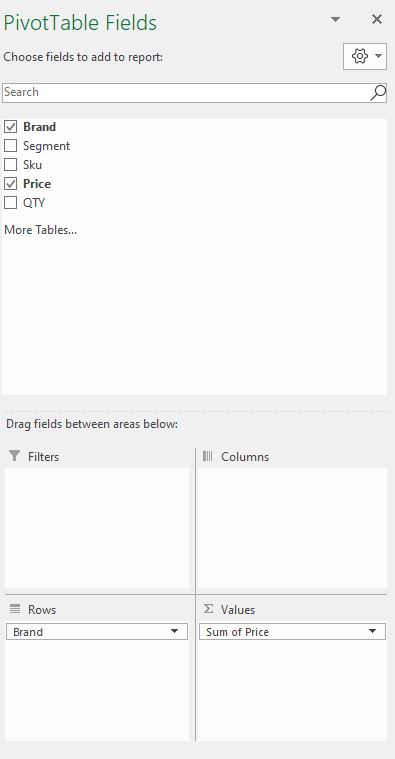
Category: PivotTablesIs this an optimal data structure to import in a Pivot table?
CorrectIncorrect -
Question 16 of 105
16. Question
Category: PowerPivot basicsWhich objects exist in PowerPivot data model?
CorrectIncorrect -
Question 17 of 105
17. Question
Category: PowerQuery basicsCombine the correct statement with keyword:
Sort elements
- PowerQuery
- M
-
User interface through which you can easily clean and transform source data.
-
Formula language that is being written for us on each interaction with the tool. You can also write it yourself in the formula bar or in Advanced editor.
CorrectIncorrect -
Question 18 of 105
18. Question
Category: Dynamic Array FormulasWhich symbol do we need to use after referencing cell containing array formula to active its #SPILL feature?
CorrectIncorrect -
Question 19 of 105
19. Question
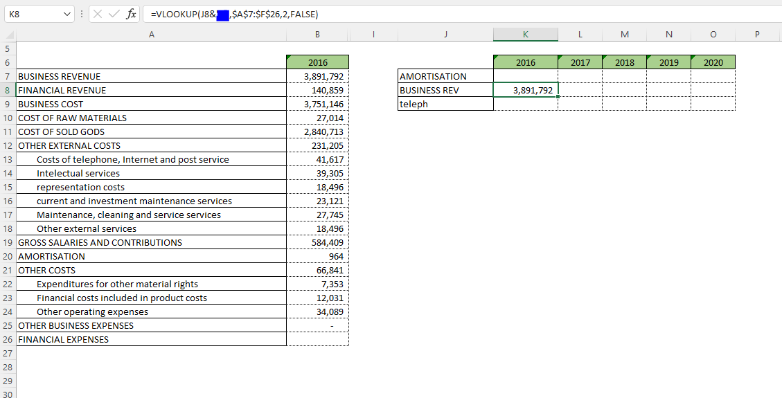
Category: PowerPivot basicsHow is the red squared cell value calculated?
CorrectIncorrect -
Question 20 of 105
20. Question
Category: PowerQuery basicsWhen considering data cleaning operations, what are PowerQuery’s advantages compared to VBA?
CorrectIncorrect -
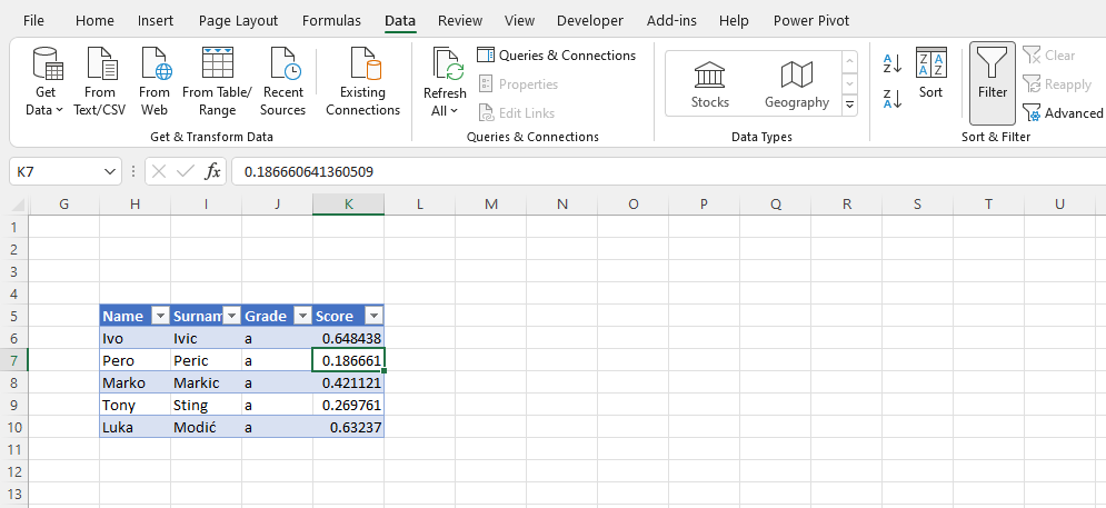
Question 21 of 105
21. Question
Category: Merging Sources (VLOOKUP, XLOOKUP, INDEX, etc.)Using the following formula in a cell K7 will yield:
CorrectIncorrect -
Question 22 of 105
22. Question
Category: Excel TablesCombine the appropriate Excel table syntax with its usage:
Sort elements
- Single column reference
- Row by row calculation using a single column reference
- Multiple whole columns absolute reference
- Single column row by row calculation with absolute referencing
-
Table1[Column]
-
Table1[@Column]
-
=Table1[[Column1]:[ColumnN]]
-
=Table1[@[Column]:[Column]]
CorrectIncorrect -
Question 23 of 105
23. Question
Category: PowerPivot basicsHow can you connect multiple tables imported in PowerPivot data model?
CorrectIncorrect -
Question 24 of 105
24. Question
Category: PivotTablesWhat are the benefits of using slicers?
CorrectIncorrect -
Question 25 of 105
25. Question
Category: PivotTablesSelect all the features that apply to PivotTables:
CorrectIncorrect -
Question 26 of 105
26. Question
Category: PivotChartsCan you create a PowerPivot chart without the PivotTable?
CorrectIncorrect -
Question 27 of 105
27. Question
Category: PowerPivot basicsWhich filters are active in the red cell?
CorrectIncorrect -
Question 28 of 105
28. Question
Category: PivotChartsWhich of the following objects can you filter using slicers?
CorrectIncorrect -
Question 29 of 105
29. Question
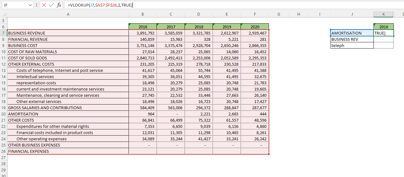
Category: Merging Sources (VLOOKUP, XLOOKUP, INDEX, etc.)You need to create a wild card search based on text in the J column. Which wildcard symbol do you need to use in the VLOOKUP function to find Business Revenue in a list of values in column A?
CorrectIncorrect -
Question 30 of 105
30. Question
Category: PivotChartsIs chart a part of Worksheet cells?
CorrectIncorrect -
Question 31 of 105
31. Question
Category: Dynamic Array FormulasUsing the Excel file you can download here, answer the following question.
You wish to add a FILTER formula that will dynamically show all table rows with a date specified in cell M3, and category specified in cell M2.
Write the correct formula using table reference (all relative refences).
CorrectIncorrect -
Question 32 of 105
32. Question
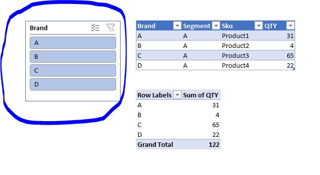
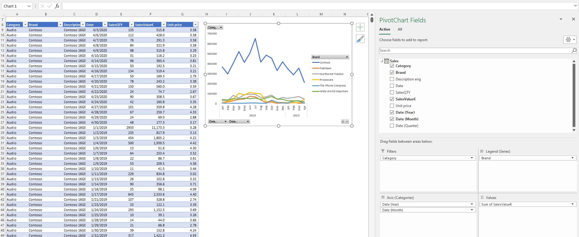
Category: PivotChartsUsing the picture below, match PivotChart fields with ColumnNames:
Sort elements
- Filters
- Brand
- Date (Year) and Date (Month)
- SalesValue€
-
Category
-
Legend (Series)
-
Axis (Categories)
-
Values
CorrectIncorrect -
Question 33 of 105
33. Question
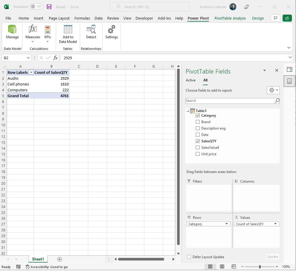
Category: PowerPivot basicsWe have a PowerPivot table plotted on a spreadsheet, like in the picture below.
Where can we check what the Table3 table data structure looks like?
CorrectIncorrect -
Question 34 of 105
34. Question
Category: Dynamic Array FormulasWe wish to create a list of unique brands from Table1 sorted in ascending order.
Which function/functions are correct?
CorrectIncorrect -
Question 35 of 105
35. Question
Category: Merging Sources (VLOOKUP, XLOOKUP, INDEX, etc.)Match the wildcard symbol with the corresponding search values (we use the # symbol to represent the needed symbol).
Sort elements
- ?
- *
- ~
-
Replaces any single symbol (eq: "Tr#y" equals with "Tray", "Troy", and "Trey", but not "Trolley")
-
Replaces any number of symbols after the symbol (eq: "Tr#y" equals also with "Trolley".)
-
Ignore Wild card (eq: "Tr#?y" equals with "Tr?y", but not with "Tray" or "Troy".)
CorrectIncorrect -
Question 36 of 105
36. Question
Category: Excel ConditionsWhich formula/s will return the correct TRUE/FALSE if cells in column B equal cells in column C?
CorrectIncorrect -
Question 37 of 105
37. Question
Category: PowerPivot basicsWhat is DAX (Data Analysis Expressions) being used for?
CorrectIncorrect -
Question 38 of 105
38. Question
Category: Dynamic Array FormulasUsing the Excel file you can download here, answer the following question.
You wish to add a FILTER formula that will dynamically show all table rows with a date specified in cell M3.
Write the formula using table reference.
CorrectIncorrect -
Question 39 of 105
39. Question
Category: PivotChartsObserve the picture below:
Source of the selected Pivot chart is:
CorrectIncorrect -
Question 40 of 105
40. Question
Category: PowerPivot basicsCan you import multiple different source tables into a single PowerPivot data model?
CorrectIncorrect -
Question 41 of 105
41. Question
Category: Dynamic Array FormulasUsing the Excel file you can download here, answer the following question.
You wish to use the SORT function to sort the whole table by Brand column in descending order.
Which formula should you use?
CorrectIncorrect -
Question 42 of 105
42. Question
Category: Excel data entryCan you clear only cell formatting without deleting cell content?
CorrectIncorrect -
Question 43 of 105
43. Question
Category: PivotChartsWhich type of charts are not supported in PivotChart?
CorrectIncorrect -
Question 44 of 105
44. Question
Category: PowerPivot basicsWhere do you input PowerPivot DAX formulas?
CorrectIncorrect -
Question 45 of 105
45. Question
Category: Dynamic Array FormulasUsing the Excel file you can download here, answer the following question.
You wish to use the SORT function to sort the whole table first by column Description eng, then by SalesValue€. Both columns need to be sorted in descending order.
Write the formula using table reference.
CorrectIncorrect -
Question 46 of 105
46. Question
Category: Dynamic Array FormulasCombine tasks with appropriate function:
Sort elements
- XLOOKUP
- SUMIFS
- SUBTOTAL
- FILTER
-
Combine data from multiple sources
-
Aggregate values based on conditions
-
Aggregate values based on filters applied
-
Return multiple rows of data based on condition
CorrectIncorrect -
Question 47 of 105
47. Question
Category: PivotChartsWhat are PivotChart benefits when compared to a regular chart?
CorrectIncorrect -
Question 48 of 105
48. Question
Category: PowerPivot basicsImport of data in PowerPivot is done through:
CorrectIncorrect -
Question 49 of 105
49. Question
Category: Excel ConditionsWhat are the differences between IF and SUMIFS functions?
CorrectIncorrect -
Question 50 of 105
50. Question
Category: Excel FormulasIf you need to enter a formula to a single cell on a worksheet, do you need to understand what referencing is (the $ signs)?
CorrectIncorrect -
Question 51 of 105
51. Question
Category: PivotTablesWhich general type of fields can you can add to a PivotTable?
CorrectIncorrect -
Question 52 of 105
52. Question
Category: PowerPivot basicsWhen importing data in the PowerPivot model, how many rows is the maximum import limit?
CorrectIncorrect -
Question 53 of 105
53. Question
Category: Excel TablesIn a proper table, can you have 2 columns with the same name?
CorrectIncorrect -
Question 54 of 105
54. Question
Category: PowerPivot basicsWhich Loading options should you choose if you wish to load the PowerQuery script only in the PowerPivot data model? (Select all that applies)
CorrectIncorrect -
Question 55 of 105
55. Question
Category: Excel FormulasIf you need to enter a formula in a cell, then copy that formula across a range of cells, do you need to understand what referencing is (the $ signs)?
CorrectIncorrect -
Question 56 of 105
56. Question
Category: Excel ConditionsDownload the following Excel workbook and use it to answer the question.
We want to add condition in D column stating that if SalesValue€ is less than 500.000€ (cell H3 value), then we apply 15% discount (cell I3 value). Else we apply 27% discount (cell I4 value).
Which formula should be entered into cell D4? The formula should show the correct result when copied across the whole D column. Use absolute references where necessary.
CorrectIncorrectHint
Use absolute referencing to cells containing percantage and condition values.
-
Question 57 of 105
57. Question
Category: PivotTablesCan you add a column to the Values field of the PivotTable?
CorrectIncorrect -
Question 58 of 105
58. Question
Category: PowerPivot basicsWhat is the source of PowerPivot table?
CorrectIncorrect -
Question 59 of 105
59. Question
Category: PivotTablesHow can you fix the width of the PivotTable columns so they do not change as you select different filters?
CorrectIncorrect -
Question 60 of 105
60. Question
Category: PowerPivot basicsMatch the correct statement with the correct Excel tool
Sort elements
- Is used to perform advanced dynamic analytics upon cleaned and well-defined data
- Is used to transform and clean messy data structures
- Is used to perform static ad-hoc analysis
-
PowerPivot
-
PowerQuery
-
Excel formula
CorrectIncorrect -
Question 61 of 105
61. Question
Category: PowerPivot basicsCombine pictures with the correct type of PivotTables:
Sort elements
- PowerPivot table
- PivotTable
CorrectIncorrect -
Question 62 of 105
62. Question
Category: PowerPivot basicsWhat are the differences between PivotTable created from the data model (PowerPivot), and regular Pivot created from table/range? Select all that apply.
CorrectIncorrect -
Question 63 of 105
63. Question
Category: PowerPivot basicsCan you add Measures to Rows or Column fields of the Power PivotTable?
CorrectIncorrect -
Question 64 of 105
64. Question
Category: Merging Sources (VLOOKUP, XLOOKUP, INDEX, etc.)In which situations could you benefit from lookup functions (VLOOKUP, XLOOKUP, INDEX, etc.)?
CorrectIncorrect -
Question 65 of 105
65. Question
Category: Excel data entryCombine Excel operations with keyboard shortcuts:
Sort elements
- CTRL+Home
- CTRL+End
- CTRL+A
- CTRL+SHIFT+ ⬇ arrow
- CTRL+ ⬇ arrow
- CTRL+Shift+End
-
Go to A1 cell on Worksheet
-
Go to the last populated cell on a worksheet
-
Select all cells in a populated range
-
Select all cells from the selected to the last populated one (rows)
-
Jump from the selected cell to the last populated one (rows)
-
Select all cells from the selected to the last populated one
CorrectIncorrect -
Question 66 of 105
66. Question
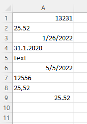
Category: Excel data entryIf there is no previous formatting applied, which rows have a text value entered in a cell? (Multiple choices)
CorrectIncorrectHint
Numbers are not always what they seem to be in Excel!
-
Question 67 of 105
67. Question
Category: Excel data entryIf there is no previous formatting applied, which rows have a text value entered in a cell? (Multiple choices)
CorrectIncorrectHint
Numbers are not always what they seem to be in Excel!
-
Question 68 of 105
68. Question
Category: Excel data entryIf there is no previous formatting applied, which rows have a correct date entered in a cell? (Multiple choices)
CorrectIncorrect -
Question 69 of 105
69. Question
Category: PowerQuery basicsIn Excel, how can we push parameter values inside of a Query?
CorrectIncorrect -
Question 70 of 105
70. Question
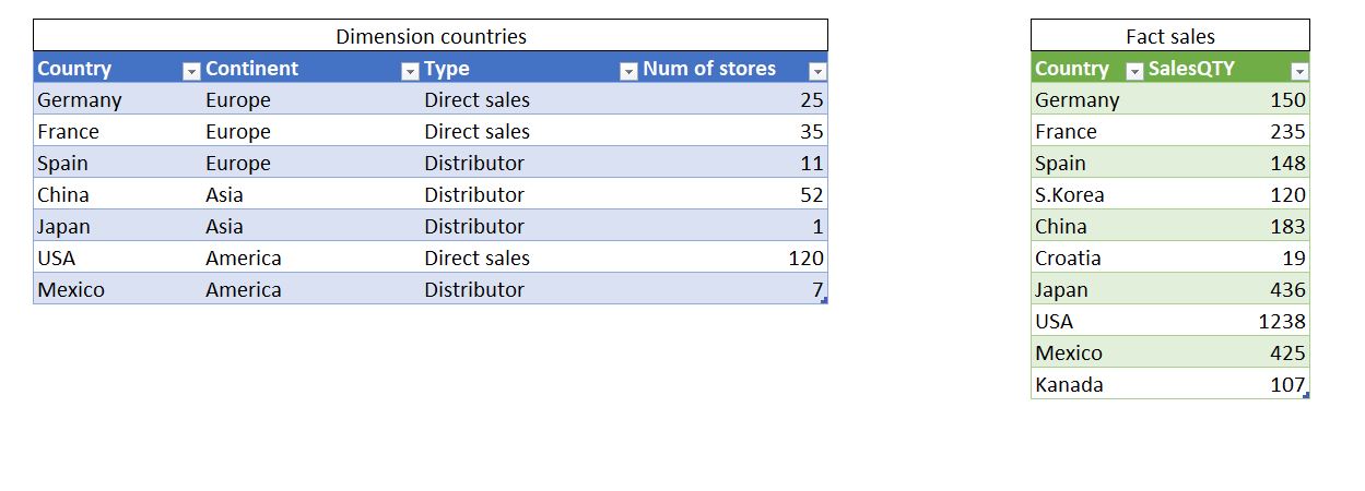
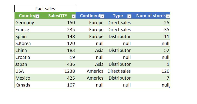
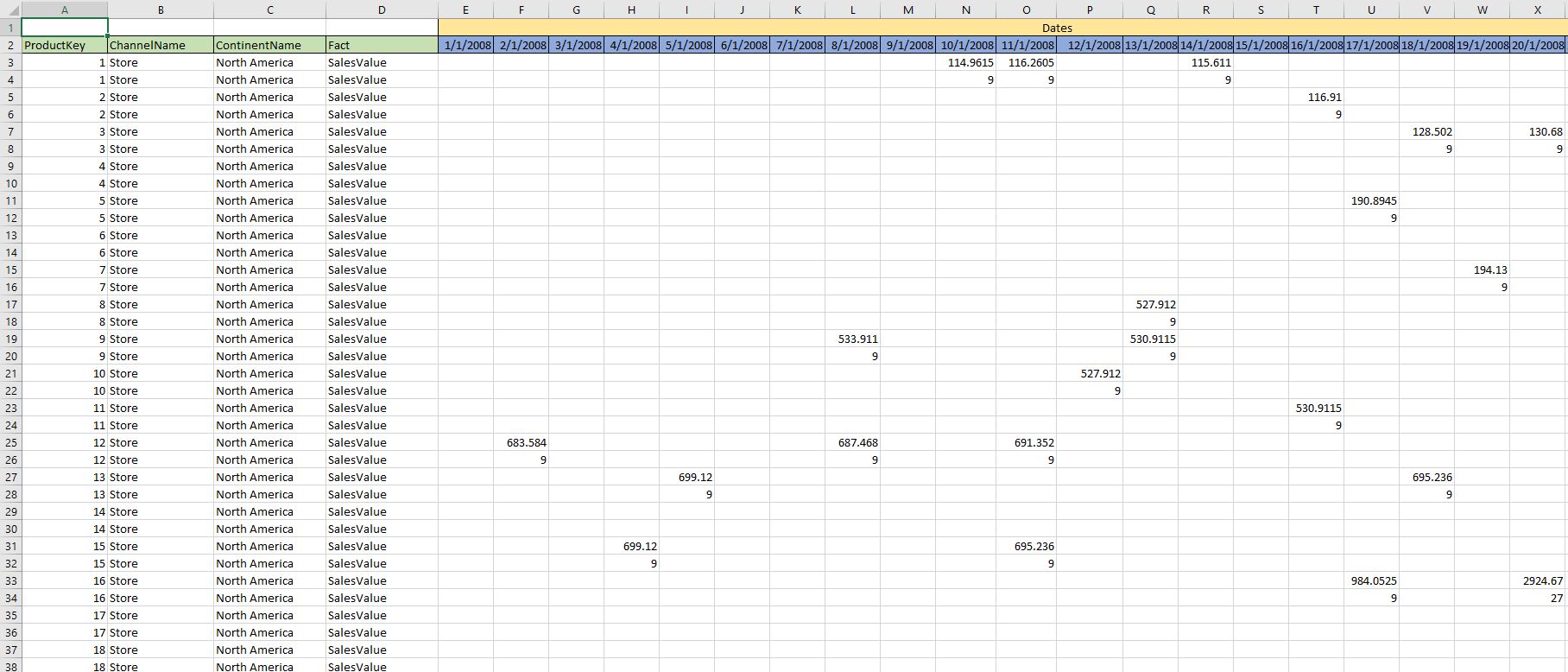
Category: PowerQuery basicsYour database consists of 2 different tables. Dimension table with a list of countries and its descriptions, and a fact table with the name of the Country and Quantity of products sold for each country.
You want to denormalize dimension descriptions in a fact table (like in a picture below).
You can see that in the merged table there are null values meaning that you have to add those countries with its descriptions to the dimension table. What is the easiest way to filter out values that exist in the fact table, but are non existing in dimension? (Picture below)
CorrectIncorrect -
Question 71 of 105
71. Question
Category: Excel data entryIf there is no cell formatting applied, match types of entry with their position in a cell (after confirming entry).
Sort elements
- Align right
- Align left
- Align middle
-
Number
-
Text
-
Errors
CorrectIncorrect -
Question 72 of 105
72. Question
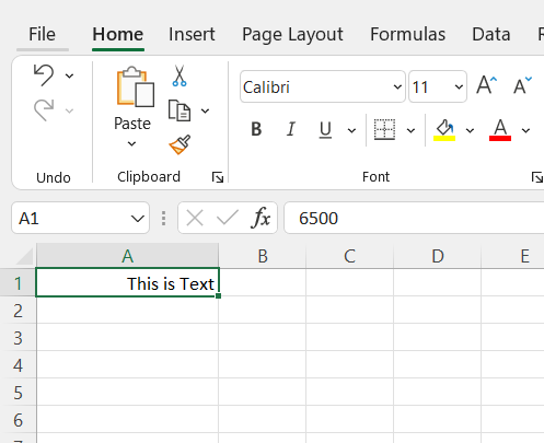
Category: Excel data entryHow does Excel interpret this entry?
CorrectIncorrect -
Question 73 of 105
73. Question
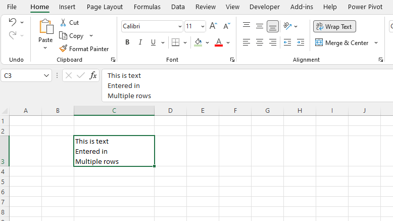
Category: Excel data entryWhich keyboard combination can split the text into multiple rows inside of a single cell?
CorrectIncorrect -
Question 74 of 105
74. Question
Category: Excel data entryCombine Excel shortcuts with appropriate cell data entry:
Sort elements
- CTRL+SHIFT+; (semicolon)
- CTRL+SHIFT+: (colon)
-
Current date
-
Current time
CorrectIncorrect -
Question 75 of 105
75. Question
Category: PowerQuery basicsWhich kind of files does binary type usually hold?
CorrectIncorrect -
Question 76 of 105
76. Question
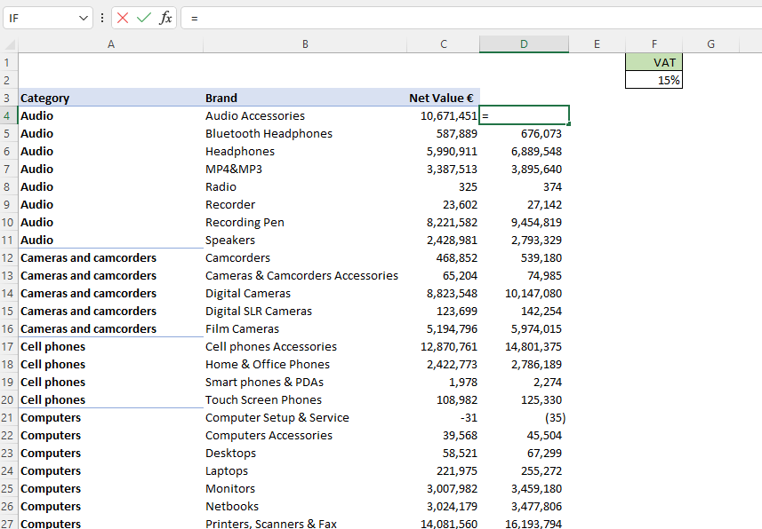
Category: Excel FormulasYou need to add a VAT (Value added tax) to each net amount.
Which is the preferred way of entering the 15% VAT.
CorrectIncorrect -
Question 77 of 105
77. Question
Category: PowerQuery basicsYou created a script in which data source is .csv document exported from your local system. You stored both data sources and PBI file containing a script on a server location that all your colleagues can access and use. After some time colleagues start sending you a screenshot like in a picture below. What happened?
CorrectIncorrect -
Question 78 of 105
78. Question
Category: Excel FormulasWhich symbol is used to lock column and/or row references when writing formulas?
CorrectIncorrect -
Question 79 of 105
79. Question
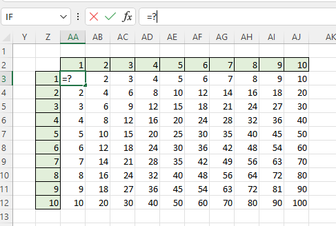
Category: Excel FormulasWe want to create a multiplication table in Excel. Which formula entered in cell AA3 will yield a correct answer when copied across the whole range (AA3:AJ12)?
CorrectIncorrect -
Question 80 of 105
80. Question
Category: PowerQuery basicsYou need to change the table in the picture below into a better modeling structure.
The optimal data structure should look like in the table below.
Which Power Query transformation do we need to run over the initial table to transform it into an optimal structure?
CorrectIncorrect -
Question 81 of 105
81. Question
Category: PowerQuery basicsPut the applied steps in the correct order to transform the data in the picture below into optimal form.
-
#"Promote Headers"
-
#"Unpivot Other Columns"
-
#"Remove Top Row"
-
#"Change Column Types"
CorrectIncorrect -
-
Question 82 of 105
82. Question
Category: Excel FormulasYou need to add a VAT (Value added tax) to each net amount.
In the input area, write the function syntax you need to enter in cell D4 so that it shows correct results across the whole D4:D1000 range (do not use spaces in formula).
CorrectIncorrect -
Question 83 of 105
83. Question
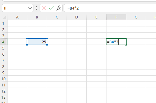
Category: Excel FormulasYou enter a formula as in the picture below:
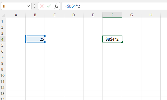
What would happen if we copy cell F4 (the one with the formula), and paste it into cell B2?
CorrectIncorrect -
Question 84 of 105
84. Question
Category: Excel FormulasYou enter a formula as in the picture below:
What would happen if we copy cell F4 (the one with the formula), and paste it into cell B2?
CorrectIncorrect -
Question 85 of 105
85. Question
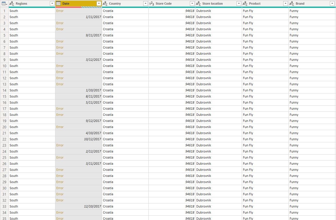
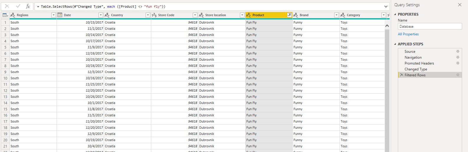
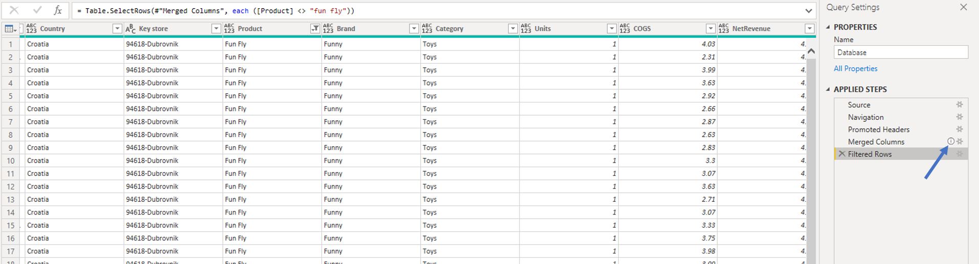
Category: PowerQuery basicsYou tried to filter out the Fun Fly product from the table, but it didn’t work (picture below). What happened?
CorrectIncorrect -
Question 86 of 105
86. Question
Category: Excel FormulasYou enter a formula as in the picture below:
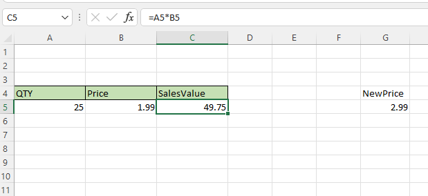
What would happen if we cut cell G5 (the one with the value 2.99), and paste it into cell B5?
CorrectIncorrect -
Question 87 of 105
87. Question
Category: PowerQuery basicsWhat does the exclamation mark icon in the picture represent?
CorrectIncorrect -
Question 88 of 105
88. Question
Category: Excel FormulasWhen we use Copy/Paste native shortcuts (CTRL+C ==> CTRL+V), what is being pasted into the new range? (Select all options that apply)
CorrectIncorrect -
Question 89 of 105
89. Question
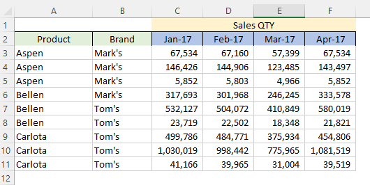
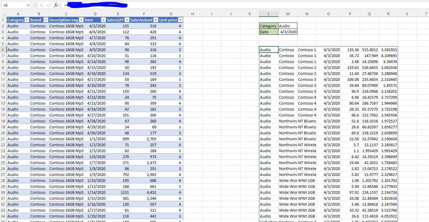
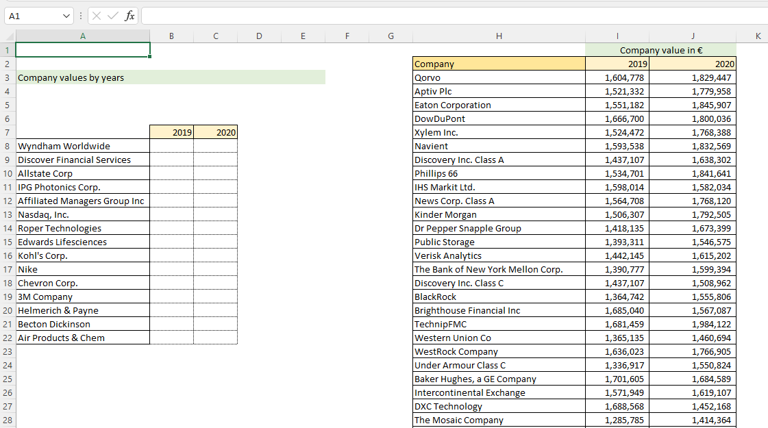
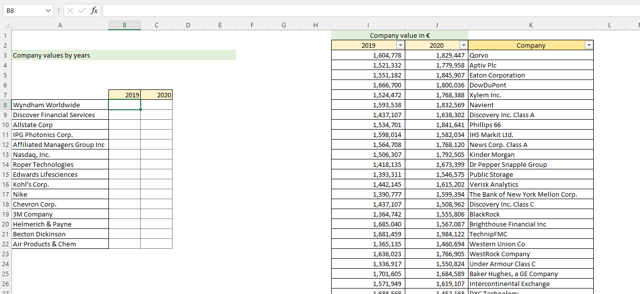
Category: Merging Sources (VLOOKUP, XLOOKUP, INDEX, etc.)For the list of companies in the left table, we need to find its corresponding values from the table to the right.
Which functions (one or more selections are correct) can help us find the correct values for years 2019 and 2020? In the table to the right, there are over 500 unique company names.
CorrectIncorrect -
Question 90 of 105
90. Question
Category: Merging Sources (VLOOKUP, XLOOKUP, INDEX, etc.)For the list of companies in the left table, we need to find its corresponding values from the table to the right.
In the table to the right, there are over 500 unique company names (list ending in row 507).
Using VLOOKUP, which function entered in cell B8 will yield a correct answer when copied across the whole range B8:C22?
CorrectIncorrect -
Question 91 of 105
91. Question
Category: Merging Sources (VLOOKUP, XLOOKUP, INDEX, etc.)For the list of companies in the left table, we need to find its corresponding values from the table to the right. We must make no structural changes to the table to the right.
Which functions (one or more selections are correct) can help us find the correct values for years 2019 and 2020? In the table to the right, there are over 500 unique company names.
CorrectIncorrect -
Question 92 of 105
92. Question
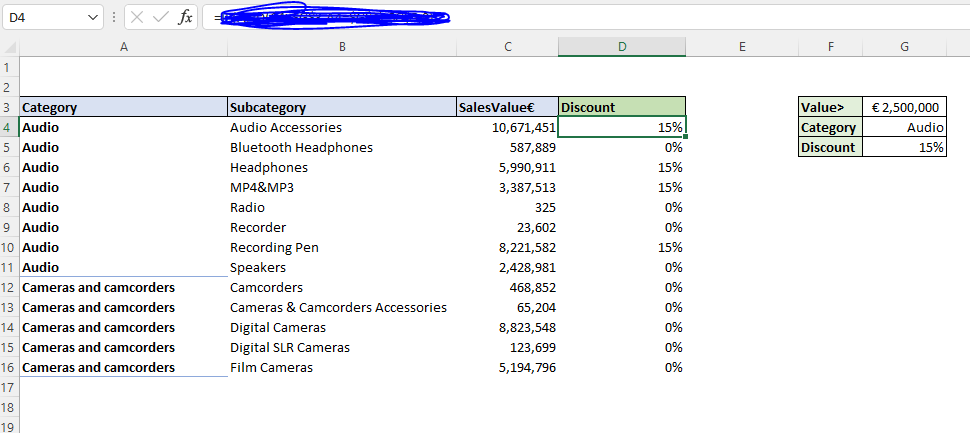
Category: Excel ConditionsWe want to give a special discount to all products coming from the Audio category if their sales exceed 2,500,000 € SalesValue.
The formula needs to work when copied across the whole D4:416 range. Which formula is the correct one?
CorrectIncorrect -
Question 93 of 105
93. Question
Category: Excel ConditionsWe want to apply conditional formatting in the table below. The condition is that for any value greater than 5.000.000 (cell H2 value), the whole row of the table needs to turn green.
Can we use any of the default circled options from the conditional formatting pane to achieve this or do we need to define a custom rule?
CorrectIncorrect -
Question 94 of 105
94. Question
Category: Excel ConditionsWe want to apply conditional formatting in the table below. The condition is that for any value greater than 5.000.000 (cell H2 value), the whole row of the table needs to turn green.
If using a custom formatting rule, which is the correct formula that will format the whole row in green in case it evaluates to true?
CorrectIncorrect -
Question 95 of 105
95. Question
Category: Excel TablesIs this a propper Excel table?
CorrectIncorrect -
Question 96 of 105
96. Question
Category: Excel TablesWhat are the main benefits of using real tables as compared to table-like structures? (Multiple choices)
CorrectIncorrect -
Question 97 of 105
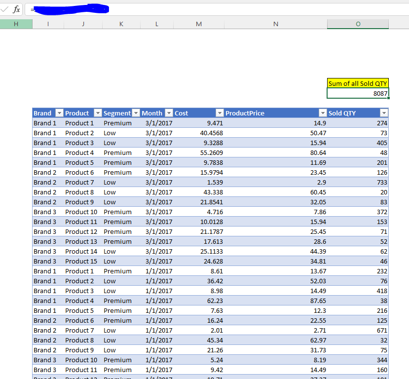
97. Question
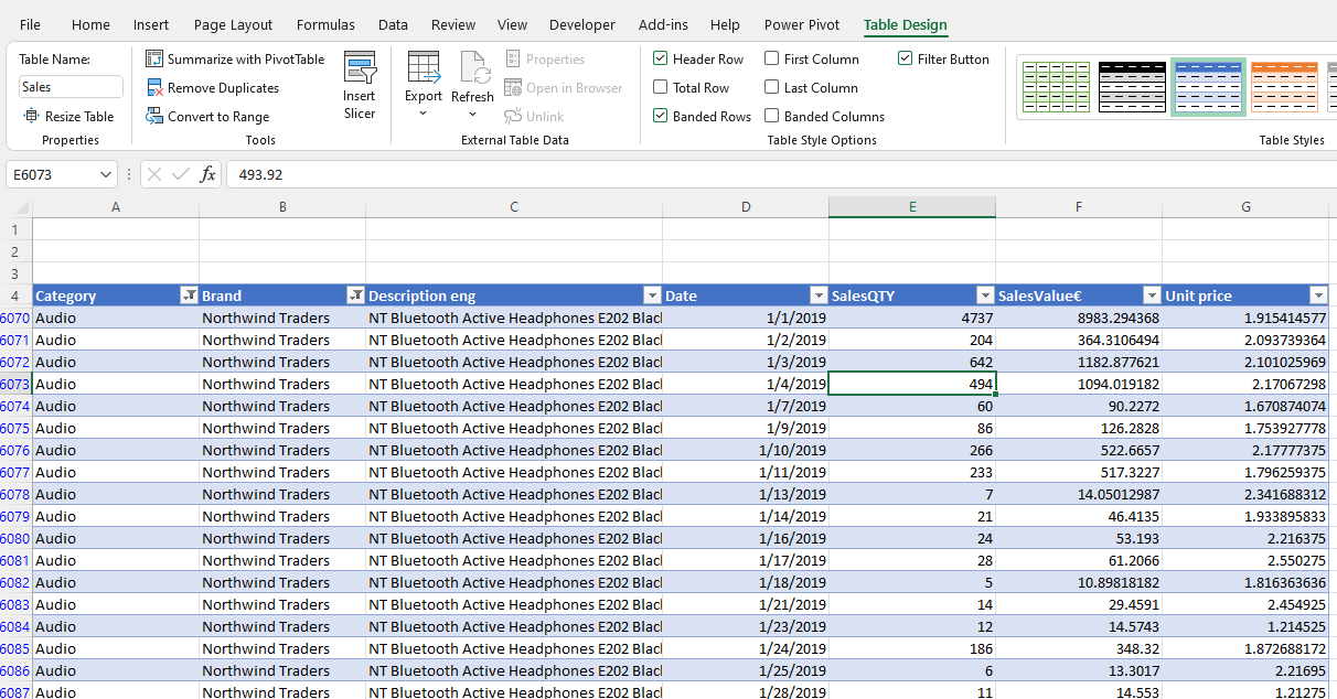
Category: Excel TablesIn Cell O8 we wish to sum all Sold QTY from the table named Sales (picture below). The last populated row in a table is row 1200.
Which formula syntax is the correct one? (One or more correct answers)
CorrectIncorrect -
Question 98 of 105
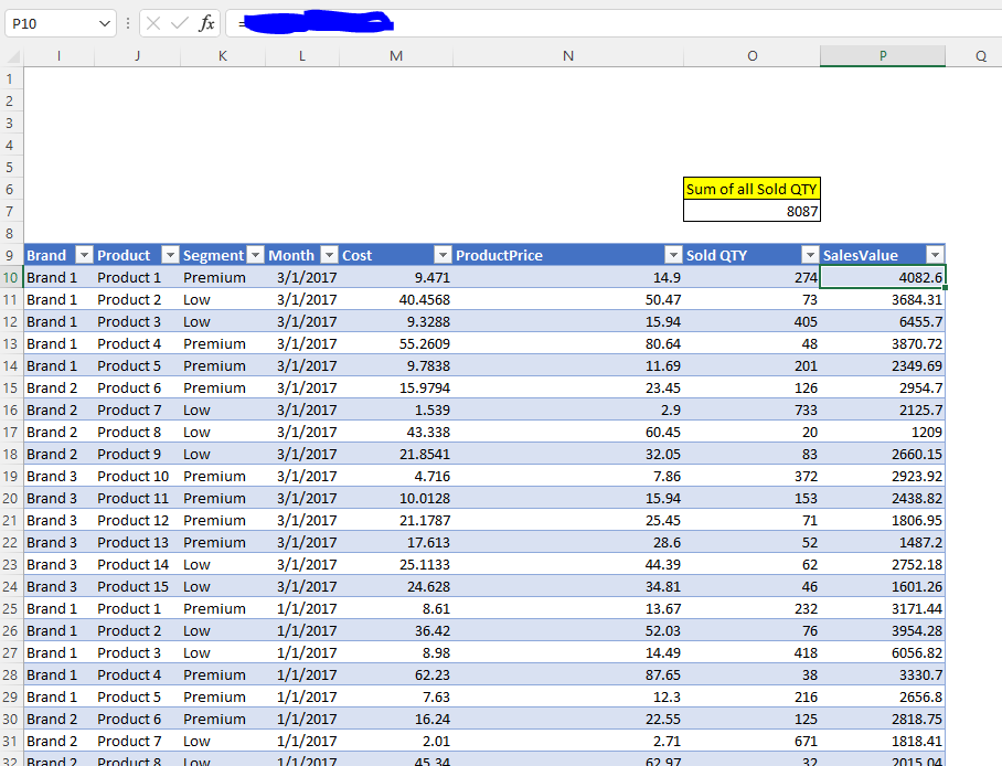
98. Question
Category: Excel TablesWe wish to add a new column to a table called SalesValue. Its formula is ProductPrice * SoldQTY.
Which formula syntax is the correct one if entered in a cell P10? (One or more correct answers)
CorrectIncorrect -
Question 99 of 105
99. Question
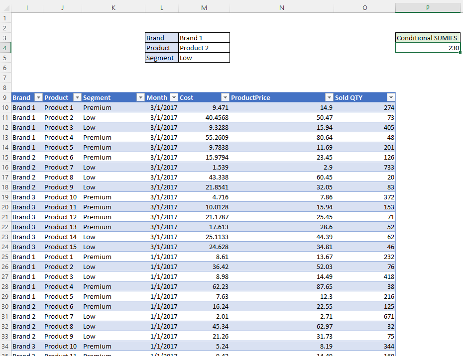
Category: Excel TablesWe wish to create SUMIFS conditional formula which sums all Sold QTY in a Sales table based on the criteria in a range L3:M5.
Both provided formulas will return the correct result. Which one is better to use?
CorrectIncorrect -
Question 100 of 105
100. Question
Category: Excel TablesWe wish to create SUMIFS conditional formula which sums all Sold QTY in a Sales table based on the criteria in a range L3:M5.
Which statements are correct if we use =SUMIFS(O:O,I:I,M3,J:J,M4,K:K,M5) formula (formula addressing whole column ranges)?
CorrectIncorrect -
Question 101 of 105
101. Question
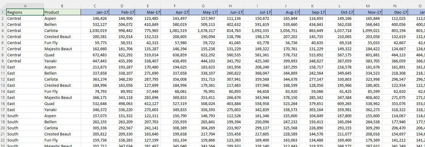
Category: Excel TablesWe wish to sum all the SalesQTY in a table Sales (picture below). We want the solution to be dynamic and to account for any newly added rows to the table (currently 21.721 rows in a table).
Sort formulas from best to worst in terms of performance and flexibility (possibility to account for newly added rows):
-
=SUM(Sales[SalesQTY])
-
=SUM(E:E)
-
=SUM(E5:E21721)
CorrectIncorrect -
-
Question 102 of 105
102. Question
Category: Excel TablesIn cell F3 we want to enter a formula that will sum only the visible table rows based on filters applied.
Which formula is correct?
CorrectIncorrect -
Question 103 of 105
103. Question
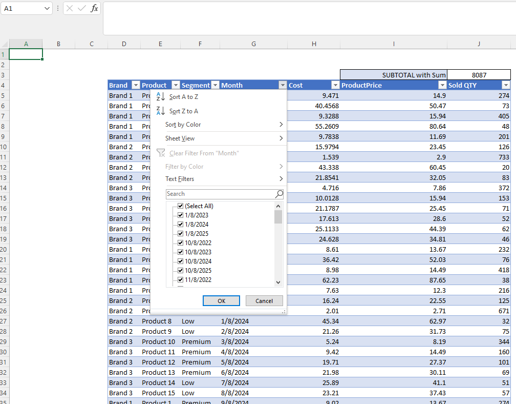
Category: Excel TablesYou want to filter the table so that it includes only sales in the year 2022. You open the filter on the date column but do not receive year selection. Instead, you receive a list of all dates.
What is wrong?
CorrectIncorrect -
Question 104 of 105
104. Question
Category: PivotTablesWhich statement about PivotTables is correct?
CorrectIncorrect -
Question 105 of 105
105. Question
Category: PivotTablesWhich statement about PivotTables is correct?
CorrectIncorrect