PivotTables, or pivoting, is by far the best analytical power of Excel. You digest the data and play with it on the fly. Heck, PowerBI is pretty much PivotTables with pretty visuals, just a lot smarter (because of DAX).
While PowerBI offers many stunning looking visuals including matrices, they do not include out of the box/easy to use pivoting experience. You could use hierarchies to some extent, but they are fixed and can only be changed while in Edit mode.

Currently, we can have a Pivoting experience in PowerBI in these ways:
- Connect through Analyze in Excel option, then create PivotTables inside Excel,
- Choose to edit apps/workspace/.PBIX files and manipulate visual fields through UI.
This is enough in case you are a creator of reports with edit rights, but in case you are only a consumer through Apps, we encounter a problem. The solutions mentioned above work only if the tenant admin allowed analyze in Excel or Apps modifications to consumers who are only viewing the content. Most of the time, in larger organizations, this is centrally managed and not set to on by default.
Why?
Even if we talk about simpler models, they tend to have around 15-20 tables, some of which are not to be used in reporting.

Only the people who author the data model know which column and measure combination produce wanted results and where to use them. Model authors might hide Measures/Tables that should not be used in the reports, but that is a tedious job for large models in development. On the other hand, if you allow anyone in the organization to pick their measures/columns, you are guaranteed to have incorrect reports down the road. Also, out of 1000 people in the organization, most of them are intimidated with the use of Pivot tables and would rather use something out-of-the-box for their quick analysis.
It would be ideal if model creators could provide a quick and intuitive way of pivoting inside the PBI by providing them with a dimension slicers which allows them to pick how to pivot their data on the fly.
In the rest of the post, we will discuss an approach to solving this issue with a Matrix visual and a 2 level depth pivoting Experience.
EXAMPLE
To start with, we will use the Sales and Marketing sample database from Microsoft. If you wish to follow along, you can download the .PBIX file here.
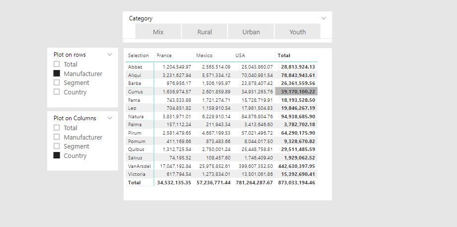
Below is an embedded example to see the pivoting in action.
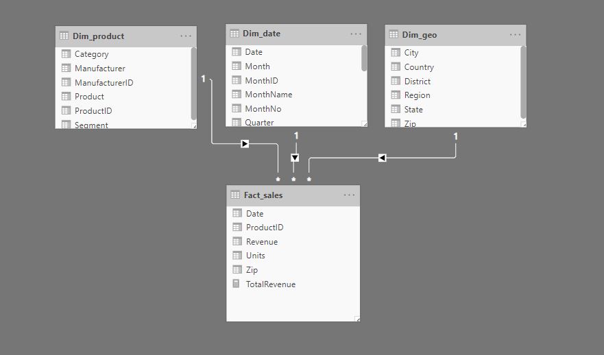
The data model is a simple one, consisting of 3 dimensions and a fact_sales table.

THE PROBLEM
We would like to be able, without the editing mode or analyze in Excel feature, choose which dimensions we want to plot in the matrix, down to 2 hierarchies. Currently, this is not natively supported with PowerBI, but can be achieved with the combination of DAX tables and measures.
THE IDEA
The idea is to provide, for each pivoting dimension, a list of key values that will filter the Fact_table on the desired granularity. We can accomplish that by creating a table inside PBI which holds the following columns: “Segmentation”, “PDC Key”, “Selection”, “Rank”, “Dimension”.
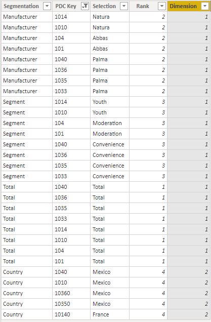
Let’s try to illustrate what each of the columns should consist of in the simplified picture below.

- Segmentation column – represent the segmentation which will be visible on the selection slicer. It should be repeated for all the Key values.
- PDC Key – the values from the Key column that form a 1 to * relationship between the dimension and a Fact_table.
- Selection column – This column represents the descriptions from the dimension table that are linked to the PDC Key value. Notice that when Segmentation is “Manufacturer” the PDC Key value 1010 is linked to Selection “Natura” (Natura is the manufacturer of 1040 product), while on “Segment” Segmentation, the same PDC Key value represents “Convenience” segment (product 1040 falls under Convenience Segment). This is the most important part of the technique. In short terms, we must repeat the same PDC Key values for all the different Segmentations, and for each segmentation, we must provide the correct description of the PDC Key.
- Rank – column used to set the ranking of the dimensions in the slicer,
- Dimension – This column needs to be used in case we wish to include segmentations coming from multiple dimension. More about this below.
At the bottom of the table, you can see that we also have a “Country” Segmentation. While all the other segmentations come from the same dimension Dim_Product, the “Country” segmentation comes from the Dim_geo dimension. Although it has the same PDC key as the product coming from Dim_Product dimension, “Country” PDC Keys represent zip codes and are not to be mistaken with Product codes. Dimension column helps us determine which relation between pivoting table and fact table we should activate. In case all our segmentations come from the same dimension, this column is not needed.
We can create this type of table from our regular dimension tables using a DAX code or with a PowerQuery. The DAX code approach below.
PivotValues1 =
VAR ALLS =
    SELECTCOLUMNS (
        ADDCOLUMNS (
            ALLNOBLANKROW ( Dim_product[ProductID] ),
            "Rank", 1,
            "Segmentation", "Total"
        ),
        "Segmentation", [Segmentation],
        "PDC Key", Dim_product[ProductID],
        "Selection", "Total",
        "Rank", [Rank],
        "Dimension", 1
    )
VAR Manufacturer =
    SELECTCOLUMNS (
        ADDCOLUMNS (
            ALLNOBLANKROW ( Dim_product[ProductID], Dim_product[Manufacturer] ),
            "Rank", 2,
            "Segmentation", "Manufacturer"
        ),
        "Segmentation", [Segmentation],
        "PDC Key", Dim_product[ProductID],
        "Selection", Dim_product[Manufacturer],
        "Rank", [Rank],
        "Dimension", 1
    )
VAR Segment =
    SELECTCOLUMNS (
        ADDCOLUMNS (
            ALLNOBLANKROW ( Dim_product[ProductID], Dim_product[Segment] ),
            "Rank", 3,
            "Segmentation", "Segment"
        ),
        "Segmentation", [Segmentation],
        "PDC Key", Dim_product[ProductID],
        "Selection", Dim_product[Segment],
        "Rank", [Rank],
        "Dimension", 1
    )
RETURN
    UNION ( ALLS, Manufacturer, Segment, Country )
EXPLANATION:
Each Variable represents one segmentation. For each segmentation (except the ALLS), we need to provide all the combinations of the PDC Key column (Dim_product[ProductID]) and the desired segmentation column (Dim_product[Manufacturer]).
Why the SELECTCOLUMNS function?
Without it, the names of the columns in the virtual table variables would depend on the names in the Dimension_table they come from. This would lead to unwanted lineage and would produce a blank result in case of mixing dimensions in the UNION part of the calculation. With the SELECTCOLUMNS function, we explicitly tell DAX how to name each column in variable tables so that they stack correctly in the union part.
To produce pivoting with 2 levels of details, we need 2 copies of the table above. We named our second copy PivotValues2. You can also include more copies of the table if you wish your pivoting to go deeper.
THE FORMULA PART
With 2 virtual tables in place, we are now able to create slicers and put related selections onto the Matrix visual. We need to tell the DAX how to read slicer related data and produce the correct results based on the Filter context.
In case all our segmentations come from the same dimension, the calculation is as follows:
RevenuePivotedSimple =
CALCULATE (
    [TotalRevenue],
    TREATAS ( VALUES ( PivotValues1[PDC Key] ), Fact_sales[ProductID] ),
    TREATAS ( VALUES ( PivotValues2[PDC Key] ), Fact_sales[ProductID] )
)
We use TREATAS function to transfer filters (PDC Key list of values) from the disconnected virtual table to the Fact table.
Formula stack both slicer selections and apply calculation in the modified filter context that is the result of the intersect of the slicers.
In case we have segmentations coming from multiple dimension tables, we need to play a bit with the formula, like in the example below.
RevenuePivotedMultyDimension =
VAR FirstDimension =
    SELECTEDVALUE ( PivotValues1[Dimension], "1" )
VAR SecondDimension =
    SELECTEDVALUE ( PivotValues2[Dimension], "1" )
RETURN
    SWITCH (
        FirstDimension & SecondDimension,
        "11",
            CALCULATE (
                [TotalRevenue],
                TREATAS ( VALUES ( PivotValues1[PDC Key] ), Fact_sales[ProductID] ),
                TREATAS ( VALUES ( PivotValues2[PDC Key] ), Fact_sales[ProductID] )
            ),
        "12",
            CALCULATE (
                [TotalRevenue],
                TREATAS ( VALUES ( PivotValues1[PDC Key] ), Fact_sales[ProductID] ),
                TREATAS ( VALUES ( PivotValues2[PDC Key] ), Fact_sales[Zip] )
            ),
        "22",
            CALCULATE (
                [TotalRevenue],
                TREATAS ( VALUES ( PivotValues1[PDC Key] ), Fact_sales[Zip] ),
                TREATAS ( VALUES ( PivotValues2[PDC Key] ), Fact_sales[Zip] )
            ),
        "21",
            CALCULATE (
                [TotalRevenue],
                TREATAS ( VALUES ( PivotValues1[PDC Key] ), Fact_sales[Zip] ),
                TREATAS ( VALUES ( PivotValues2[PDC Key] ), Fact_sales[ProductID] )
            )
    )
EXPLANATION
First, we need to catch dimensions we selected inside the slicer. We use variables for that.
Second, we need to use SWITCH to provide the CALCULATE with the correct TREATAS function depending on the dimensions selected with the slicer. The formula becomes cumbersome to write after 3 pivoting dimensions since you need to provide every possible TREATAS combination. Formula would be much easier to write if DAX IF function could return tables, but at the moment this is not possible.
The calculation can be modified and expanded to include more levels of pivoting depth or more dimension from which selection in slicer can be made. Unfortunately, each additional dimension/pivoting depth introduce complexity and slows down the calculation. There are also some considerations to be made before using this technique:
CONSIDERATIONS
- There must be no values the Key column in the Fact table that does not have a representative key in the dimension. We are using TREATAS function to transfer filters, therefore any value in the key column in the fact table that does not have a corresponding value in the dimension will simply be ignored (in case there is a physical 1 to * relationship we would see a blank line in the matrix with values not linked to dimension. With TREATAS we would not see a blank line, therefore we would have missing values in the report.)
- Cardinality of the dimensions impact overall calculation speed – up to 1000 key values ok, 1000 -10000 bit slow, 10000-100000 slow, >100000 use with caution
- A number of dimension and pivoting depths impact performance. 2 pivoting depths ok, more use with caution.
IMPORTANT!
The same technique can be achieved with — (weak relationships) between filtering tables and a fact table. In most cases, this could be a faster method. In my test model, the speed of calculation is similar using both approaches. In case this technique is slow in your model, try weak relationships.
Do not mix both techniques (either don’t connect pivoting tables and use TREATAS function to transfer filters or connect through weak relationships and use USERELATIONSHIP function in case of mixing dimensions).
Hope you enjoyed reading through the post and that you liked this technique. In case of any questions, please comment below!


