Gradimo softver kakav vaša tvrtka priželjkuje
Moderniziramo način na koji poslujete - zamjenjujemo zastarjele alate i nefleksibilne low-code aplikacije skalabilnim sustavima. Prilagođeni softver, AI, automatizacija i Microsoft tehnologije, odabrani za dugoročnu vrijednost.

Rješavamo operativne probleme izgradnjom modernih poslovnih sustava
Bilo da je pravo rješenje Power Platform, prilagođeni softver ili hibrid, biramo tehnologiju koja stvara najveću dugoročnu vrijednost, a ne trend trenutka.
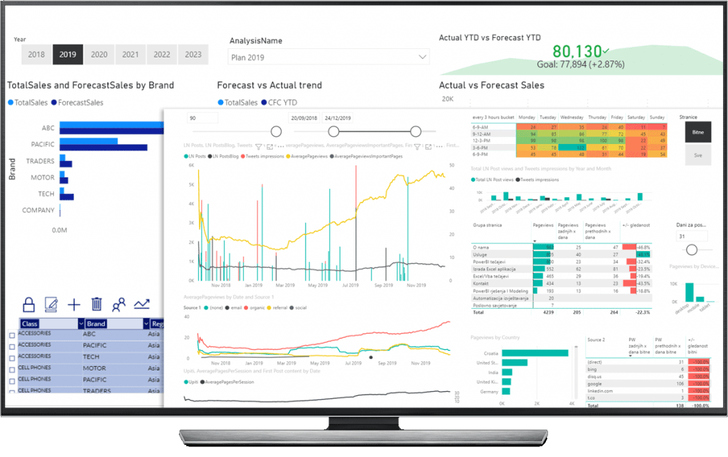
PowerBI / Fabric
Dashboardi, izvještaji i moderna data platforma koja sirove podatke pretvara u sigurne odluke.
Saznaj više →PowerApps
Prilagođene poslovne aplikacije koje povezuju vaše timove, podatke i procese.
Saznaj više →Edukacije (Akademija)
Praktične edukacije uživo za početnike i profesionalce, koje vode certificirani predavači.
Saznaj više →Poslovne i tehnološke konzultacije
Konzultacije uživo i online, utemeljene na poslovnom iskustvu i dubokom poznavanju Microsoft platforme.
Saznaj više →Writeback Planner za PowerBI planiranje
Gotovo writeback rješenje za planiranje koje budgetiranje i forecasting donosi izravno u Power BI.
- Writeback planiranje izravno u vaš model
- Napravljeno za financije, budgetiranje i forecasting
- U primjeni kod 100+ domaćih i inozemnih klijenata

Benedikt - računovodstveni kontroling i analiza
Napredni Power BI sustav koji RDG, bilancu, bruto bilancu i novčani tok generira automatski iz vašeg dnevnika knjiženja.
- Automatski financijski izvještaji iz knjiženja
- Analiza do razine pojedine transakcije
- Konsolidacija više tvrtki unutar klastera
Novosti i savjeti
Vodiči za Power BI, Excel i podatke - te što je novo u Exceedu.
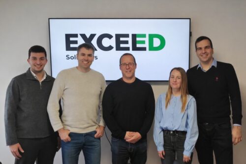
Ponovno smo proširili naš tim!
Exceed nastavlja rasti - upoznajte najnovije članove našeg BI tima.
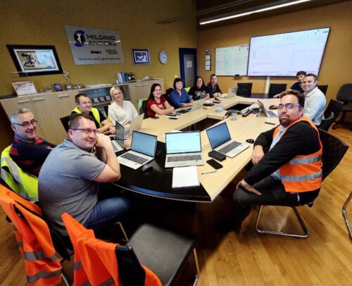
Napredna Excel edukacija za klijenta Hilding Anders
Prilagođeni napredni Excel program za međunarodnog proizvođača.

Glavne greške budgetiranja u Excelu
Uobičajene zamke budgetiranja - i kako ih Power BI pomaže izbjeći.
Unaprijedite svoje vještine - za početnike i profesionalce
📢 Naši tečajevi preselili su se na Udemy. Power BI, Power Query i Excel tečajevi vlastitim tempom sada su dostupni na Udemyju - učite kad god i gdje god želite.
Već ste kupili ovaj tečaj na našoj staroj stranici? Pošaljite e-mail na academy@exceed.hr i naši moderatori akademije poslat će vam besplatni Udemy kupon.
Pogledaj tečaj na Udemyju →Pogledajte kako predajemo
Besplatni Power Query i Power BI videi - uvjerite se u naš stil poučavanja prije nego se prijavite na tečaj.
Na YouTubeu od 2020. · Novi videi redovito
Za sve dodatne informacije, kontaktirajte nas putem forme
Opišite nam svoj izazov s podacima i javit ćemo vam se s prilagođenom ponudom.