
Power Query, or Get&Transform in Excel 2016, is an ultimate tool for data transformation before loading it to Excel/Power BI.

PowerQuery stands as a mediator between different data sources (Databases, Excel files, Web sources…) and final input. We can say that it acts like a macro recorder, but instead of recording movement across sheets, it records transformation steps applied to the source before importing structured and clean data into Excel for further analysis.
In Excel 2016 PowerQuery is already included as a standard part of Excel and can be found under Data Tab => Get&Transform Data group. If you are using Excel 2010/2013, you can download it as a free Add-in. Just follow this short tutorial.

What are the benefits of using PowerQuery instead of simply pasting data in excel and making all the necessary adjustment in it?
The biggest advantage of using PowerQuery versus manual data manipulation in Excel is speed and efficiency.
Imagine you have daily/weekly/monthly reporting, and for each of these, you receive data from different sources. Of course, data rarely comes nicely formatted, and almost always require additional shaping before becoming somewhat acceptable for report creation. So, every time you receive new data, you must manually apply all transformation steps which take a significant amount of time and increase errors. I have seen people spending three days a month on refreshing presentations with most of that time spent transforming data to useful formats. PowerQuery eliminates manual steps, giving you more time to do what you are paid for, which is finding insights from data.
Another big advantage of PowerQuery it that it can to connect to almost any kind of data source, and retain a connection to it. This way, when new data comes, all you need to do is click on a refresh button. Refresh and transformation part work together, so whenever you refresh data, all transformation steps are applied, eliminating manual work. Transform only once and use it always. Sounds great, right?!
Besides automation and amazing connection possibilities, PowerQuery has additional amazing features which come handy when manipulating data. I will list few of them that I consider important. Note that I am working with Excel 2016, so some parts could be slightly different in 2010/2013 version, but logic is the same.
1. Unpivot Data:
You have been thought that PivotTables are a great tool, so why Unpivot anything? Actually, this feature is designed to work in favor of PivotTables and shows very useful when you have multiple columns of data of the same type. It’s easier to show than explain, so let’s start by looking at the table below.
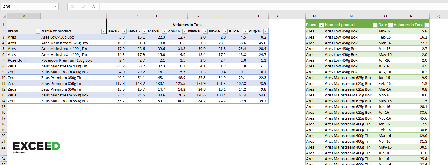
In the first table, each month is in a separate column. This is not an optimal structure of data, and you would want to get a structure more like in Table 2(right one in the picture above). In Table 2 all months are put in the same column, having only one column containing their values. This way you are reducing the number of columns and making your table more flexible.
For more technical info about Unpivoting you can check this practical tutorial.
Whenever you have a possibility to reduce the number of columns with Unpivot, you should do so. Why?
- You can apply filter/slicer to Unpivoted columns
- Data grouping is easier if all values are in the same column
- If you have all the dates in one column, you can use Time Intelligence Formulas
- It is easier to switch dimensions in PivotTable
2. Append/Combine tables
If you are receiving same data structures in multiple files (like text or CSV files) on regular basis, you will surely benefit from this feature.
To bring this concept closer to you, imagine the following scenario.
Company X needs to track employee workload and satisfaction, so they come up with an idea to create a folder on OneDrive for Business in which, each week, employees paste their last week workload/satisfaction results. You need to join that files into one report. Each week you have to open newly added Excel files and copy/paste data into your master file. Imagine having 300 employees, that is quite a big workload on weekly basis, not to mention a big chance of making an error while consolidating data.

With PowerQuery, you can create a consolidated report from all these files with a few mouse clicks. To achieve this, use Get Data From Folder option. All files from the selected folder will be imported and from there on you can apply transformation steps. If you have any files that should not be imported, you have an option to deselect them while importing.
Go to data tab, click on Get data, and select to open data from a folder. Find your folder and click ok.

A pop-up window will show up, and as soon as You press Combine&Load, you master data is ready for further analysis.

To get this simple combine to work without additional transformations, data in each Excel/Text File should be in form of tables, like in the picture below.

When new files are added to the folder, they are also automatically added to your master data. All you need to do is to refresh a Master table to insert new file records.
Combine feature allows combining all sorts of different files, so if you are really interested in more advanced solutions, you can check the links below to find more about it.
Youtube videos:
3. Merge Tables
Merge table function can completely remove the need for a VLOOKUP function. The VLOOKUP function is one of the most important functions in Excel and is good to use it as often as you can. But when used on large sets of data (few hundreds of thousands of rows) it tends to become slow and impacts file size. When dealing with large data sets, consider using PowerQuery Merge feature for faster and easier table lookup.
If you have sales data about different products, and you want to add custom segmentations to it (again, we are talking about hundreds of thousands of rows), this task would need an IT assistance or, if data is below 1 mil rows, very slow Vlookup/Index-Match formula.
Using Merge tables feature you can accomplish this task with almost no impact to file size or execution speed. Let’s take a deeper look at it with an example below. If you want to follow along, please download this sample workbook.
First, you need to bring both tables into a PowerQuery. Select one table and click on “From Table/Range” icon. This will immediately run PowerQuery window and import first table to PowerQuery.

You can easily add the other table within the PowerQuery interface. Go to New Source => Excel File => locate your working file and select second table to import.

After you imported both tables to PowerQuery editor, select main table(table1_2), then go to Merge Queries => Merge Queries as New

Pop-Up Window will appear. Select Table1 from the second drop down. Now you need to select the column on which you want to do a lookup (Name of product column) in both tables. As soon as you select desired columns, they should turn green. Choose Left Outer Join and confirm.

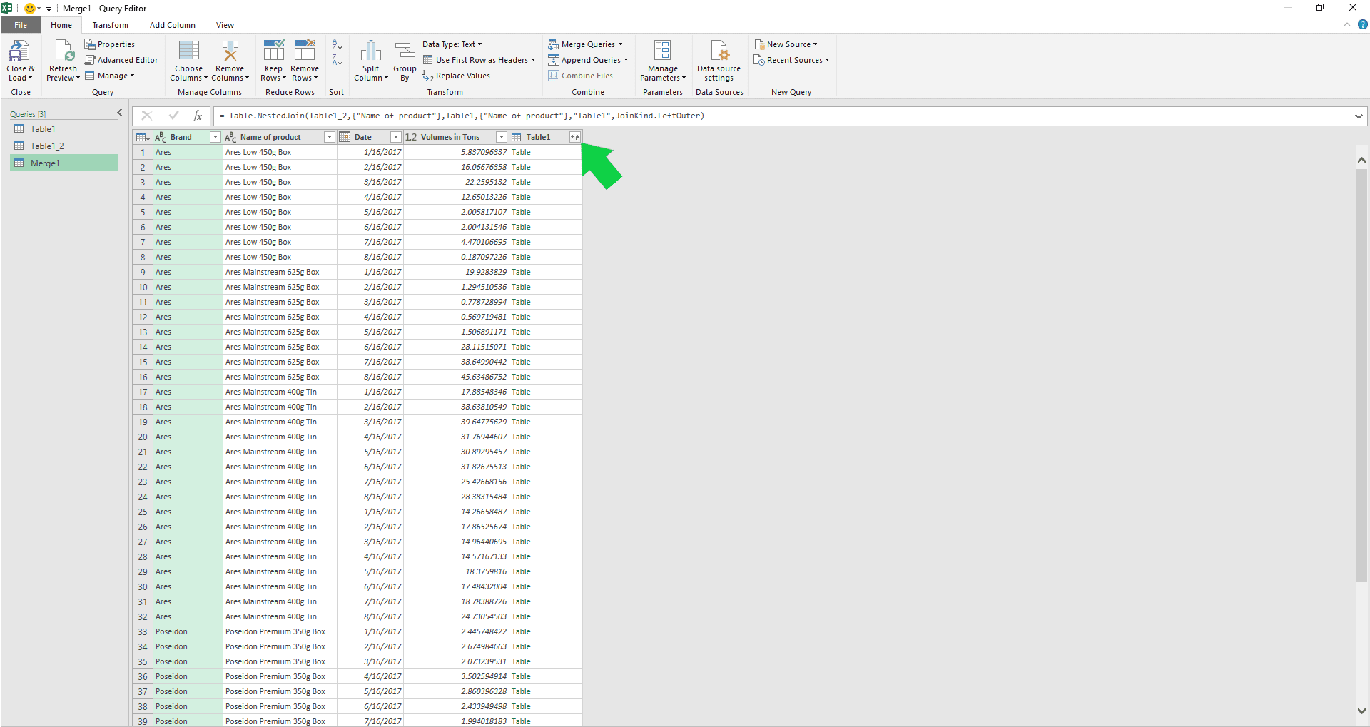
You created a new merged table named Merge1 (you can rename it to your needs). You can now select which data from lookup table you wish to import into the main table. To do that, click on splitting arrows icon in “Table 1” column of the Merge1 table.
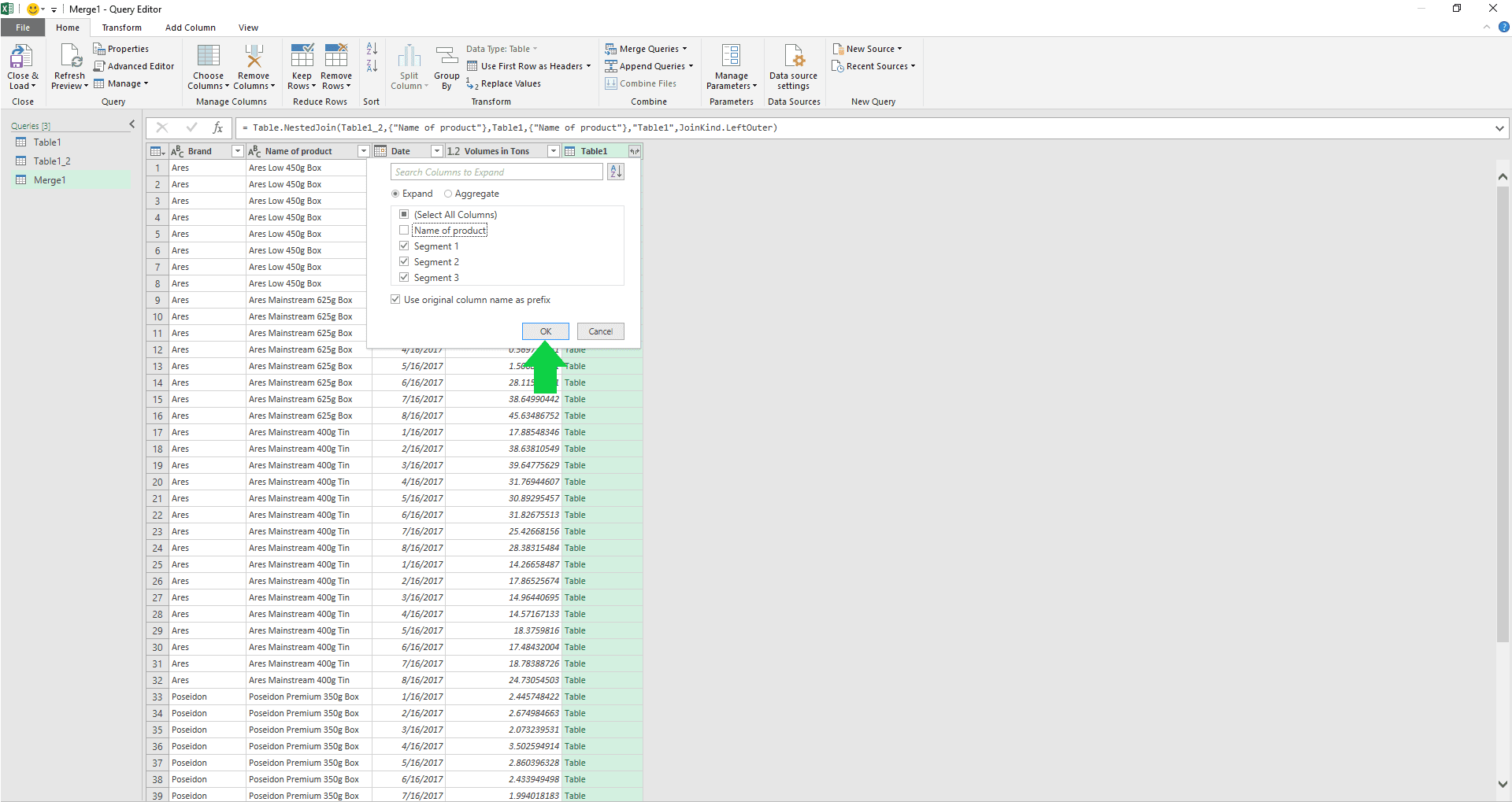
Now select all columns you wish to lookup in the main table. You can unselect Name of the product since you already have that column in the main table. Confirm with OK.
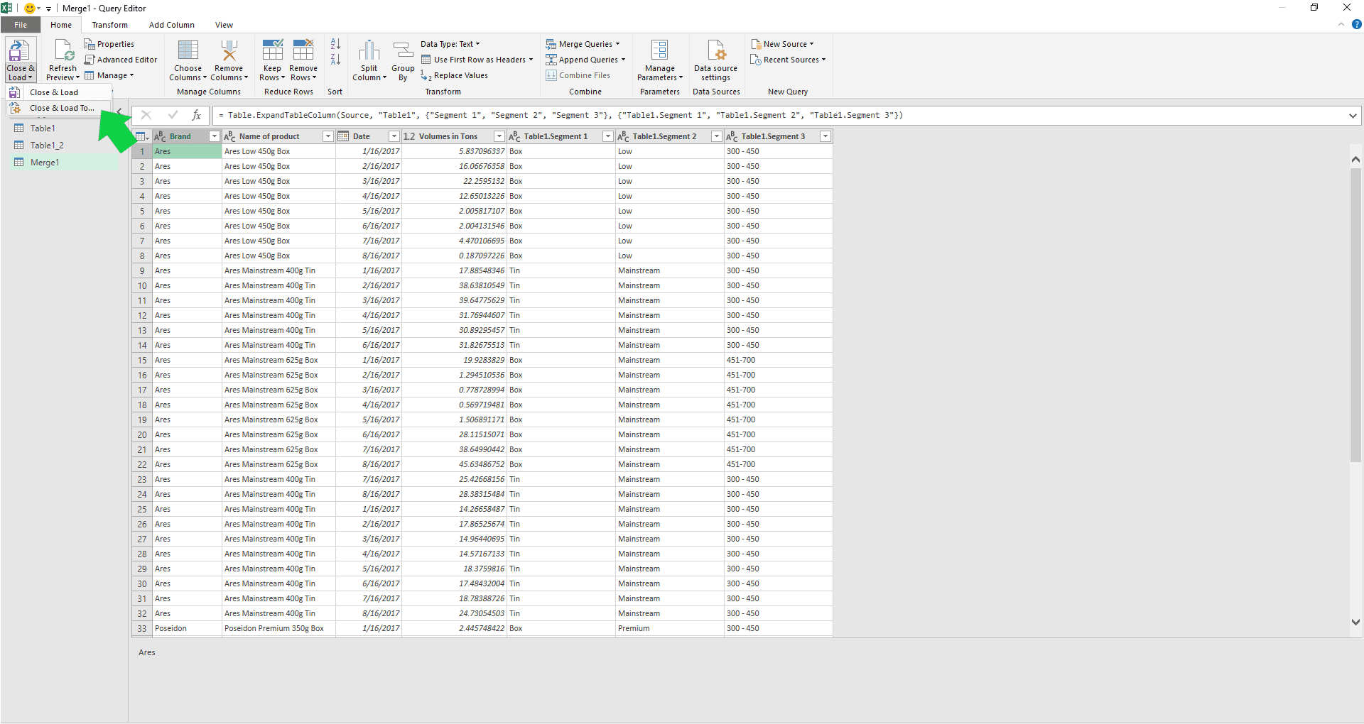
You can now add final adjustment (change column names to something more appealing, filter values, set column value types etc.). After you apply all changes, go to Close&Load => Close&Load to…=>
Different options for loading will appear. I will shortly explain each of them:
- Table – data of Merge1 table will appear on new sheet/selected range,
- PivotTable/PivotChart – PivotTable with Merge1 table as a source will appear on new sheet/selected range,
- Only Create Connection – this will not load data on your sheet or in your PivotTable, but you will be able to access this data through newly created PivotTables.
If you are building more sophisticated tables that should combine different sources, or you are making a data model, make sure you check “Add this data to the Data Model”.

Conclusions
After reading through the article, you should have a wider understanding of PowerQuery possibilities and cases in which it helps you do your work faster, easier and more precise.
You should consider using PowerQuery whenever you:
-
Do a manual transformation of data coming on regular basis (Daily, Weekly, Monthly) before using data in analysis or reporting,
-
Need to constantly ask your IT department to pull out newest data which you copy/paste into your working file. Why do that, when you can simply connect to a table stored on the server and refresh data whenever needed?
-
Have a lots of files with the same structure coming from multiple entities and you need to consolidate inputs,
-
Have large tables where you do Vlookup or Index/match.
Hope you enjoyed reading the article! if you have any questions, please comment below!
And if you liked this article, don’t forget to like/share!