
When filtering data by date, we can simply use a date slicer which is enough in most cases. We rarely need to filter our data by hours and minutes. However, sometimes this approach is necessary for the sake of the analysis.
In this blog, we will examine the scenario where we need to include hours and minutes of the day in our filtering conditions, but only for the first and the last day. For example, if we want to observe the period between 1st of January and 5th of January, from 9:30 AM (1st Jan) to 8:15 PM (5th Jan), we want to take into consideration the complete period between (full 24 hours for 2nd, 3rd and 4th Jan) and only relevant hours for the 1st Jan (from 9:30 AM to the end of the day) and the 5th Jan (from 12 AM to 8:15 PM). If we were to apply a simple filter that includes dates from 1st to 5th, and time from 9:30 AM to 8:15 PM we would lose all the data from the middle 3 days that are not in the filtered hours period. This means if there was a transaction that occurred on 3rd Jan at 8 AM, it would not be included in our analysis.
To avoid this, we will provide the solution by using DAX with a measure that will filter hours only from the relevant days (first and last one). If you wish to follow along, you can find the .pbix file on this link.
The scenario
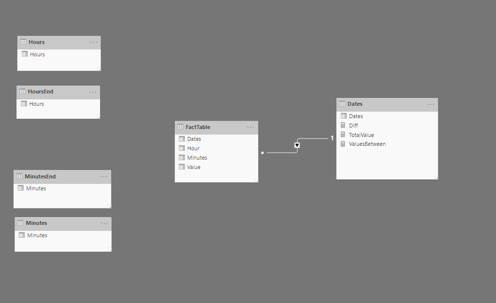
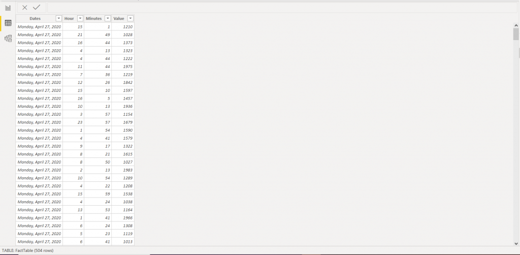
In our data model, we have a fact table that contains data with sales value and timestamp.
The Dates, Hours, and Minutes tables contain only one column which will serve for the filtering purpose. The Dates table contains all necessary dates, the Hours table contains 24 rows with values from 0-23, and the Minutes table contains 60 rows with values 0 to 59.
The HoursEnd and MinutesEnd tables are duplicates of Hours and Minutes table.
The solution
The DAX measure we will be using for this scenario:
ValuesBetween =
VAR StartDate =
    VALUE ( MIN ( Dates[Dates] ) )
VAR EndDate =
    VALUE ( MAX ( Dates[Dates] ) )
VAR StartingHour =
    FORMAT ( MIN ( Hours[Hours] ), "00" )
VAR EndingHour =
    FORMAT ( MAX ( HoursEnd[Hours] ), "00" )
VAR StartingMinute =
    FORMAT ( MIN ( Minutes[Minutes] ), "00" )
VAR EndingMinute =
    FORMAT ( MAX ( MinutesEnd[Minutes] ), "00" )
VAR StartString = StartDate & StartingHour & StartingMinute
VAR EndString = EndDate & EndingHour & EndingMinute
RETURN
    SUMX (
        FILTER (
            FactTable,
            VALUE ( FactTable[Dates] ) & FORMAT ( FactTable[Hour], "00" )
                & FORMAT ( FactTable[Minutes], "00" ) >= StartString
                && VALUE ( FactTable[Dates] ) & FORMAT ( FactTable[Hour], "00" )
                    & FORMAT ( FactTable[Minutes], "00" ) <= EndString
        ),
        FactTable[Value]
    )
Let’s take a deeper look and examine the DAX code for ValuesBetween measure.
With the 8 variables, we want to achieve the combination of numbers that gives us the right number to filter dates. Every date has its integer that represents the date value. For example, the value for the date 1/1/2020 is 43831. The value for the 1/5/2020 is 43835.
Starting and Ending hour variables are simple to understand. They are values that are formatted to always have 2 digits. For example, 4 AM is 04, and 4 PM is 16. The same logic applies for minutes.
Now, after we examined the first six variables, we can take a closer look at the StartString and EndString variables that are later used as a filter condition in our measure.
These 2 variables will always contain 9 digits that represent timestamp as an integer. For example, we will take 1/1/2020, 9:30 AM. The start string will contain StartDate, StartingHour, and StartingMinute concatenated together (StartDate = 43831, StartingHour = 09, StartingMinute = 30). StartString value, in this case, is equal to 438310930. If we go ten minutes ahead (9:40 AM), the Start string would be 438310940. This means that the StartString increased by 10 (we get the numbers that represent value and are comparable).
The EndString contains EndDate, EndingHour, and EndingMinute. For the date 1/5/2020, 8:15 PM is 438352015. If you move slicer to a few hours earlier, e.g. 5:15 PM, the value is 438351715 (lower than the first value).
We can see the idea behind the StartString and EndString. We use variables to manipulate with date, time, and hour values to get integers which are later used to compare different dates and time values.
The final point of this code is using SUMX to get the total value for the specified period of time. In SUMX function, we filter the fact table in the way that for each row, we concatenate date value, hour, and minute (based on the same logic that we applied for the StartString and EndString variables), and filter it based on conditions stated earlier in variables. This way, only the rows that are between two integers (in our earlier example, all integers between 438310930 and 438352015) pass the filtering condition.
The final test
Now let’s examine this on another example in Power BI to see if our measure works correctly.
In the table on the right, we have TotalValue that is a sum of values that take into account only date filters (without time filters), ValuesBetween, and Diff (TotalValue – ValuesBetween). On the left side, we are using 5 slicers to filter, one for date and two for hours and minutes to select the period of observation. Hours (from) and Minutes (from) slicers are coming from Hours and Minutes tables, and Hours (to) and Minutes (to) come from HoursEnd and Minutes End tables.
We can see that the values for the first and the last date for these two measures are different, and the values in the dates between are identical. This means that our code works well, and it provides a way to filter only marginal dates in our analysis.
Be careful when using this technique with big tables. Since there is a high materialization happening at a query time, you can expect degraded performance on large tables. We could further optimize this calculation by using SUMMARIZE() function instead of a whole table as a first SUMX() argument, but that is another topic about optimization.
Also, this technique does not work with built-in time intelligence functions such as DATESYTD, SAMEPERIODLASTYEAR, DATEADD, etc.
Hope you find this solution helpful in your work!
In case you have any comments, please post them below!