Dynamic ABC analysis in DAX-variables

ABC analysis is one of the most commonly used categorization techniques. This technique divides subjects of analysis (Products, Customers, Inventory, etc.) into different categories based on subject importance.

The analysis is based on the Pareto principle which states that the most economic productivity comes from only a small part of the economy. It is mainly used with large datasets with lots of different attributes. The goal is to break large datasets into three strategic segments based on their importance. This way it is easier to focus on the vital parts of your company business.

This article will demonstrate few use cases with ABC using DAX in PowerPivot.

The idea behind Dynamic ABC formula

The focus will be on explaining the dynamic pattern with the use of variables, while the static pattern is well covered in the following article by DAX maestros Marco Russo and Alberto Ferrari.

For demonstration purposes, we will use the Sales and Marketing sample database from Microsoft. If you wish to follow along, you can download the .PBIX file here.

The idea of the article is to show you how to implement different types of ABC analysis, but alongside that also to teach you parts of intermediate DAX based on the provided examples.

To be able to do a dynamic ABC analysis we need to create a table of cumulative% of the products on the fly. In static ABC analysis we could store cumulative% in a calculated column, but since we want it dynamic, we need to create a virtual table inside the DAX formula, which will be evaluated at query time (meaning each time we filter dimensions, the table will be recalculated).

The model

The data model is a simple one, consisting of 3 dimension tables, fact table, and one parameter table.

The formula

First, let’s observe the code we will use to show TotalRevenue split by the ABC clusters. It is basically a variation of the dynamic pattern by Gerhard Brueckl, just with the use of variables for better code readability. We will also use the base of this code to create [ABC NumOfProducts] measure.

ABC Granular =
CALCULATE (
    [TotalRevenue],
    VALUES ( Dim_product[Product] ),
    FILTER (
        CALCULATETABLE (
            VAR BasicTable =
                ADDCOLUMNS ( VALUES ( Dim_product[Product] ), "ProductRevenue", [TotalRevenue] )
            RETURN
                ADDCOLUMNS (
                    BasicTable,
                    "Cumulative%",
                        DIVIDE (
                            SUMX (
                                VAR CurrentProductRevenue = [ProductRevenue]
                                RETURN
                                    FILTER ( BasicTable, [ProductRevenue] >= CurrentProductRevenue ),
                                [ProductRevenue]
                            ),
                            CALCULATE ( [TotalRevenue], VALUES ( Dim_product[Product] ) )
                        )
                ),
            ALL ( Dim_product[Product] )
        ),
        [Cumulative%] > [MinBoundary]
            && [Cumulative%] <= [MaxBoundary]
    )
)

In the code we also use 3 simple measures which are:

TotalRevenue =SUM ( Fact_sales[Revenue] )

MinBoundary =MIN ( SegmentationTable[Min Value] )

MaxBoundary =MAX ( SegmentationTable[Max Value] )

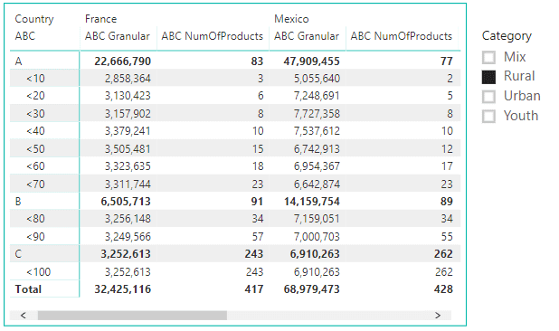
When we put [ABC Granular] and [ABC NumOfProducts] measures on a table, we get a result as shown below.

Before we start explaining the formula remember that to really understand how DAX computes its values, you have to start thinking in DAX terms. You know that the formula is the same, yet its producing different results for each field in the table. That is because in each field there are different filters applied to the data model prior the evaluation of the DAX code. So when you get a wrong result in a visual, don’t try to understand relations between figures on visuals, just focus on one single value and try to determine how it is computed in the background.

Before DAX even starts to evaluate the expression, PowerPivot model first filters the tables (and through relationship propagation the entire data model). E.q for France sales in A segment, there are two direct filters applied before formula evaluation. there is a filter coming from column header, which is France, and Youth category coming from Slicer. As we recall, segments are coming from parameter table, meaning that it cannot filter data model through relationships, but it can be used as a FILTER function argument to further restrict the data model.

From the paragraph above remember this sentence: Only after all direct filters apply the original filter context, does the PowerPivot start to Evaluate the DAX formula!

Formula evaluation

Each formula has its own evaluation order mostly impacted by the use of CALCULATE/CALCULATETABLE. The important thing to remember is that these functions have different evaluation order compared to other DAX functions. They evaluate first argument (measure or a table) only after all filter arguments are applied! you can find more about the CALCULATE evaluation order here.

With evaluation order in mind, lets split the formula into steps and explain each of them.

We will start from the outermost CALCULATE expression.

Applied steps:

0. Original filter context coming from visuals

1. CALCULATE function needs to evaluate [TotalRevenue] measure, but before doing so, it needs to accept two filters which will be joined by AND logic.

The first filter argument is VALUES( Dim_product[Product] ), which gives a list of products as visible in the current filter context (which is the original one). We need this argument to restore original filter context on Dim_product[Product] column in case we wish to use it in a report. This will be explained in details later on. 2. The second filter argument is FILTER function 3. FILTER function receives a table expression as the first argument, so before evaluating below conditions based on parameter table

[Cummulative%] > [MinBoundary] && [Cummulative%] <= [MaxBoundary]

,engine has to retrieve a table expression. 4. Table expression consists of CALCULATETABLE function wrapped around the inner part of formula. CALCULATETABLE first evaluates filter argument, which is ALL( Dim_product[Product] ), and then uses this argument to modify original Filter context for the inner table functions evaluation. This way table functions under step 4 and 5 will ignore original context filters coming from Dim_product[Product] column and will be able to compute correct cumulative totals in case we plot Dim_product[Product] column on a visual.

Filter argument of a CALCULATETABLE function is an important part of the formula because by changing it you can specify under which conditions will the cumulative% be calculated. If you change the argument ALL( Dim_product[Product] ) to ALL( Dim_product ) then cumulative% will ignore any filter coming from Dim_product table (e.q Category filter coming from slicer, like in a picture below). 5. After the filter contexts is modified by the CALCULATETABLE, formula starts to build virtual table with Cumulative%. First, we declare a table variable BasicTable, which consist of two columns:

Column containing a list of products - VALUES ( Dim_product[Product] ) 6. Column with total revenue of each product (created by ADDCOLUMNS function) 7. Previously created BasicTable variable is used in step 5 to create cumulative% inside a virtual table. To create cumulative% we need to divide running products total with the total revenue of all the products. To accomplish that we need to do the following.

On the table variable we add a virtual column called Cumulative% (using ADDCOLUMNS function) 8. For each row in virtual Cumulative% column we evaluate formula inside DIVIDE() function.

Numerator: to get the running total as numerator, we need to iterate through all the products and sum only the ones that have >= revenue compared to the current product. In DAX terms this is done as follows:

Before we enter nested row context by invoking FILTER function, we store the total revenue of the currently iterated row (the one of the cumulative% calculated column) in a variable CurrentProductRevenue. 9. FILTER function creates nested row context over the BasicTable, then iterates through it and checks which products in nested table have >= ProductRevenue compared to CurrentProductRevenue (the revenue stored in a variable of the outer row context). When FILTER finishes, SUMX function sums the ProductRevenue of the rows remained after filtering. Since there is a nested row context you can also use EARLIER function to achive the same result. 10. Denominator

We used CALCULATE with VALUES filter argument to return total revenue of all the products in the selection. 11. After table functions evaluate their expressions we receive a virtual table like the one below.

If you need to create a virtual table in your DAX code, but are unsure how the table looks like, you can install DAX studio to help you write a query against your data model (you can’t do this directly in PowerBI or Excel). This way you can easily manipulate your code inside studio environment until its ready to be used as filter argument in DAX formula. For more information about DAX studio, please follow this link.

Filling the gaps in the formula

Now that we got to the innermost part of the formula and received our virtual table, we start returning to the original outermost CALCULATE to provide it with second filter argument. If we look at the step num 2, we can see that FILTER part still has to evaluate conditions over the table returned by the CALCULATETABLE function.

Final step: Rows in the virtual table that survive FILTER conditions will be used as second filter argument to the outermost CALCULATE function.

I believe 2 things in the final step need additional explanation

1. Why do we need to use VALUES( Dim_product[Product] ) as the first argument to CALCULATE?

• The second argument to CALCULATE is CALCULATETABLE which removed the filter from Dim_product[Product] column. By doing so it removed the original filter context in case Dim_product[Product] column is to be plotted on a visual. Without the VALUES( Dim_product[Product] ) as the first argument, when we plot Dim_product[Product] column on the visual, we would see all the products with the same value (the value of the TotalRevenue of all the products in observer segment). With the use of VALUES( Dim_product[Product] ), because of the AND logic of filter arguments, we are restoring the original filter context of the products column.

1. Why is CALCULATETABLE table even a valid filter expression for the CALCULATE function?

• As we know, second filter argument is a virtual table, so then why does it provide the right set of products to filter Fact_sales table? The short answer is that virtual tables, in most cases, retain a lineage (connection) to the tables they originate from. In this case, a virtual table retained its lineage to Dim_products table, and through propagation was able to filter Fact_sales table, like in the picture below.
• 
• Although virtual tables never truly materialize inside the data model, at the query time they act just like regular tables (in case their columns preserve lineage). Lineage topic is well explained here.

Dynamic ABC variations

Counting the number of Products in each category

If you wish to count how many products there are in A,B or C segment, you can do that with the following formula.

ABC NumOfProducts =
VAR OriginalProducts =
    FILTER ( VALUES ( Dim_product[Product] ), [TotalRevenue] > 0 )
RETURN
    COUNTROWS (
        FILTER (
            FILTER (
                CALCULATETABLE (
                    VAR BasicTable =
                        ADDCOLUMNS ( VALUES ( Dim_product[Product] ), "ProductRevenue", [TotalRevenue] )
                    RETURN
                        ADDCOLUMNS (
                            BasicTable,
                            "Cumulative%",
                                DIVIDE (
                                    SUMX (
                                        VAR CurrentProductRevenue = [ProductRevenue]
                                        RETURN
                                            FILTER ( BasicTable, [ProductRevenue] >= CurrentProductRevenue ),
                                        [ProductRevenue]
                                    ),
                                    CALCULATE ( [TotalRevenue], VALUES ( Dim_product[Product] ) )
                                )
                        ),
                    ALL ( Dim_product[Product] )
                ),
                [Cumulative%] > [MinBoundary]
                    && [Cumulative%] <= [MaxBoundary]
            ),
            Dim_product[Product] IN ( OriginalProducts )
        )
    )

This formula is the same as the original one, just wrapped inside COUNTROWS function instead of being used as a filter argument in CALCULATE.

Applied steps:

0 – Original filter context coming from visuals

1. We first need to store a list of products with revenue >0 into a variable table called OriginalProducts. This way we are eliminating products that don’t have sales but would have been counted in C segment because their cumulative% is <=1. COUNTROWS function is waiting for the table argument.
2. The FILTER function is receiving table from step 3 and filtering it so that only rows with ProductRevenue >0 survive. The IN syntax is used to create a list of values that are valid for the given column. In this case, the IN syntax provides a dynamic set of OR statements with the same column. You can find more info about the IN syntax here.

Final step: After the virtual table is filtered so that it contains only products with revenue >0, COUNTROWS function can calculate the correct number of products in A,B, and C segment.

Providing a letter for each product based on its ABC segment.

The following example is a bit trickier. Instead of counting or summing products, we want to provide, for each product, a letter associated with the segment it belongs to, like in the picture below.

This way we can easily spot product importance across different dimension like regions, periods etc. Formula is a rather complex one.

ABC Show Letter =
VAR OriginalProducts =
    FILTER ( VALUES ( Dim_product[Product] ), [TotalRevenue] > 0 )
RETURN
    MINX (
        FILTER (
            CALCULATETABLE (
                VAR BasicTable =
                    ADDCOLUMNS ( VALUES ( Dim_product[Product] ), "ProductRevenue", [TotalRevenue] )
                RETURN
                    ADDCOLUMNS (
                        ADDCOLUMNS (
                            BasicTable,
                            "Cumulative",
                                DIVIDE (
                                    SUMX (
                                        VAR CurrentProductRevenue = [ProductRevenue]
                                        RETURN
                                            FILTER ( BasicTable, [ProductRevenue] >= CurrentProductRevenue ),
                                        [ProductRevenue]
                                    ),
                                    SUM ( Fact_sales[Revenue] )
                                )
                        ),
                        "ABC",
                            CALCULATE (
                                VALUES ( SegmentationTable[ABC] ),
                                FILTER (
                                    SegmentationTable,
                                    [Cumulative%] > [MinBoundary]
                                        && [Cumulative%] <= [MaxBoundary]
                                )
                            )
                    ),
                ALL ( Dim_product[Product] )
            ),
            Dim_product[Product] IN ( OriginalProducts )
        ),
        [ABC]
    )

Explanation:

To accomplish the desired result, we need to add an additional column to the virtual table inside CALCULATETABLE funtion containing a letter for each product based on its Cumulative%. This time we will start explaining the formula from the last step.

Step 3

1. We add an additional column to the virtual table using ADDCOLUMNS function
2. For each row in the newly created column, we check the boundaries of cumulative%. Since the filter part of the CALCULATE function in step 3 is designed to return only rows with one distinct value for the SegmentationTable[ABC] column from the SegmentationTable, the main argument of CALCULATE - VALUES( SegmentationTable[ABC] ) will automatically transform that distinct value to a scalar ( A, B or C).

Step 2

1. The FILTER function is receiving the virtual table and filtering it so that only rows with ProductRevenue >0 survive (Products stored in OriginalProducts variable).

Virtual table returned in step 2 looks like the one below.

Step 1

MINX function takes the virtual table as the first argument and, respecting the original filter context, returns the letter associated with the current product.

You would have thought that MINX can only return numbers, but in fact, since it always returns only one minimal value from the values supplied in the column, it automatically transforms that value into a scalar.

In case you use this formula at the granularity greater than product, it will return the smallest letter from the array of letters valid for the current context, like in the example below.

Changing the formula behavior

As I mentioned at the beginning, you can alter all these formulas to suit your specific needs. In case you wish to alter the contexts in which cumulative% is calculated, you can play with the filter argument of the CALCULATETABLE (dark colored line in the code below).

If you want to further split your ABC analysis (for example by 10%), you can create parameter table like the one in the example and use different columns to further divide segments. The segmentation table should look like this.

Now you can acquire results like in the picture below where you can see a further split of values and number of products accounted for each 10% of sales.

The variations of these formulas are numerous and can fit your specific needs with only a few adjustments (basically just one line of the code).

Hope you enjoyed reading this article. If you have any questions please comment below!

And if you liked the article, don’t forget to like/share!