Explanation
When we talk about filtering directions, we are referring to the arrows in the relationships.

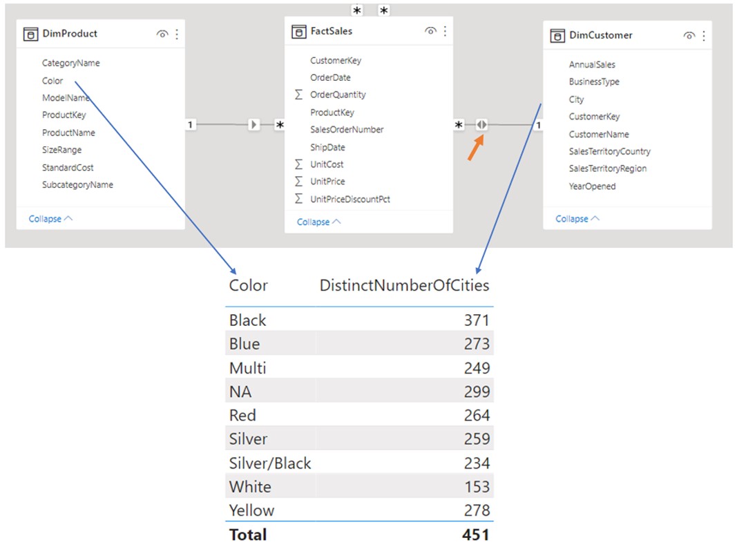
The way they are pointing is the way the filters can move through the data model. Most of the time you will have a single way of filtering data, and that is from 1 to many side of the relationship (the left orange arrow in the picture above). You can also allow bidirectional filtering, meaning filters can move from many to one side of the relationship too (the right orange arrow).
Single Filter Direction
Let’s say we want to calculate the distinct number of Cities our products are sold in.
The calculation we will use is
DistinctNumberOfCities = DISTINCTCOUNT(DimCustomer[City])
We will first try with a single-direction filter.

We want to show [DistinctNumberOfCities] filtered by the Colors column coming from DimProduct Table.

The result is always the same number, which is the total number of Cities in the DimCustomer table. Even though there is a relationship between the two tables through the FactSales table, the filters are unable to access the DimCustomer table through the relationship FactSales[CustomerKey] -> DimCustomer[CustomerKey] because the arrow is pointing only in the direction of the FactSales table. This means that filter can travel from DimCustomer to the FactSales table, but the opposite direction is not possible, so the filter reaches the FactSales, but when it has to “jump” onto DimCustomer one, it is stopped. Since no filter reaches the DimCustomer table, the values for each color are DistinctCount of DimCustomer[City] with no filters applied.
Setting Cross-filter Direction to Both
Now let’s change the direction between the tables and observe the results.

This time the calculation shows the expected figures. The filter from the DimProduct table can reach the DimCustomer table and is able to filter its row so that only the ones corresponding to a specific color survive. We will now explain in detail the internals of the filter flow for the [DistinctNumberOfCities] calculation. We will focus only on the row in the visual containing filter “Black”.
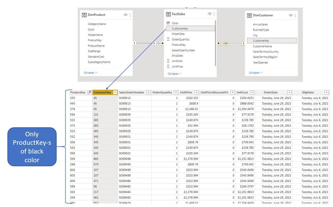
The Black filter on the Color column filters the DimProduct so that only black color rows survive.

In the Fact table, Product keys that survived condition “= Black” color cross filter CustomerKeys column. Only CustomerKeys of products with Black color will survive and will form a list of CustomerKeys which will jump to the DimCustomer table and filter it.

Crossfilter is a special DAX capability to form a list of active values for column based on filters applied to different columns of the same table. In the example above. We can see that black color will filter out certain ProductKeys from FactSales table. Those product keys will have only corresponding CustomerKeys survive the filtering. CustomerKeys that survive based on ProductKey filter are the one who are being crossfiltered.
After the DimCustomer is filtered so it contains only CustomerKey-s of sales of Black products, does the calculation kick in and count distinct values of the column City of the rows that survived the condition.

The distinct count of the column City for the Color “Black” equals 371 and that number is returned to the corresponding cell in the visual.
Use Cases
Using bidirectional filters is not a good idea, especially on high cardinality columns, since it tends to slow down calculations and can also introduce ambiguity in a data model. It’s often a better idea to always keep the filtering direction from 1 to many sides, and apply bidirectional filters only when strictly needed for specific calculations with the use of CALCULATE function. The same calculation could be written the following way, without the need for applying a bidirectional filter on the relationships.
DistinctNumberOfCitiesCalculate =
CALCULATE(
    DISTINCTCOUNT( DimCustomer[City] ),
    CROSSFILTER ( FactSales[CustomerKey], DimCustomer[CustomerKey], BOTH )
)
CROSSFILTER is a CALCULATE modifier function that can activate different types of relationship filtering directions. Those directions can be:
- Both
- None
- One Way
- One Way left to right
- One Way right to left
The advantage of using CROSSFILTER function instead of activating bidirectional relationship is flexibility to use bidirectional filters only in specific calculations and without potential negative impact on the whole data model.
Active vs Non-active
Data Model takes good care of relationships, especially with regard to Ambiguity. Ambiguity means that filters can travel from one table to the other through 2 or more different paths. In the picture below we can see that there are two possible paths between DimDate and DimCustomer tables. One is through the Fact table, and the other is a direct connection through many 2 many relationship based on Year columns. In this case, the model automatically makes one of the relationships non-active. But we can activate it on demand with the use of CALCULATE + USERELATIONSHIP function modifier.

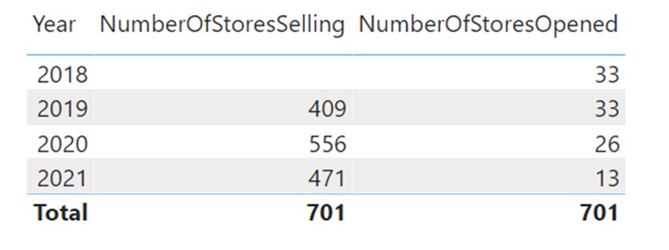
We will add 2 calculations and observe their results.
NumberOfStoresSelling = COUNTROWS(DimCustomer)
NumberOfStoresOpened = CALCULATE(COUNTROWS(DimCustomer),USERELATIONSHIP(DimDate[Year],DimCustomer[YearOpened]))

[NumberOfStoresSelling] is using active relationships in the model, going through the FactSales table to reach DimCustomer and perform the calculation. [NumberOfStoresOpened] measure uses CALCULATE modifier USERELATIONSHIP to activate the direct M2M relationship between DimDate and DimCustomer, therefore, ignoring the active relationship path.


