6.3. Row 2 Filter context transition
Explanation
Context transition is one of the most powerful features of CALCULATE function. Whenever we use CALCULATE inside of a row context (iterative functions like SUMX, FILTER, or in a calculated column), CALCULATE transforms row context to filter context.
What is the difference?
In row context, values from the current row of the iteration can only see their own row, and cannot be used as filters for other rows or tables. When we transform row 2 filter context, we are making all the values of each row become filters that can travel through the model and filter it. This feature is much easier to explain through the following example:
TopQTYWrong = MAXX(VALUES(FactSales[SalesOrderNumber]),SUM(FactSales[OrderQuantity]))
TopQTYCorrect = MAXX(VALUES(FactSales[SalesOrderNumber]),CALCULATE(SUM(FactSales[OrderQuantity])))
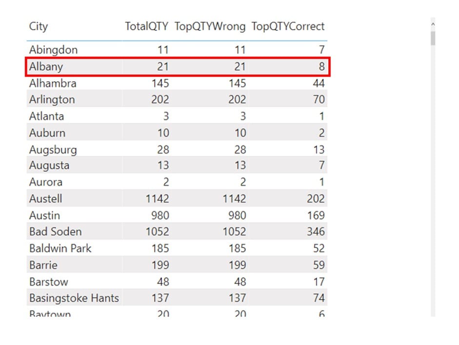
We want to calculate the top selling order for each City in the data model. Each order might consist of more lines of products, so we need to iterate through each order, sum its values and then return the order which has the highest OrderQuantity. We will focus on Albany city.
The FactSales table, when filtered to Albany city, looks like this:
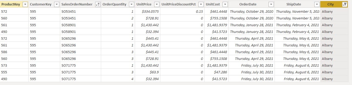
We can see that there are 4 orders in this city, each consisting of multiple lines of data. First, let’s explain the wrong calculation which returns the same figure as the [TotalQTY] measure.
No Context Transition
TopQTYWrong =
MAXX(
    VALUES( FactSales[SalesOrderNumber] ),
    SUM( FactSales[OrderQuantity] )
)
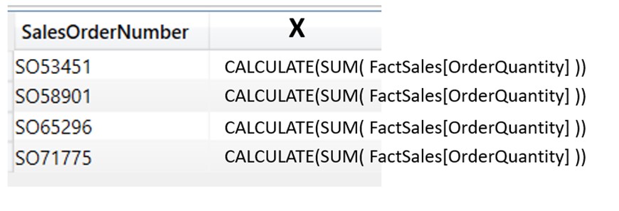
- MAXX function is adding a virtual X column to the table created with VALUES function, and that table holds 4 SalesOrderNumbers, as shown in the picture below:

- The X part of the MAXX calculation is the expression SUM( FactSales[OrderQuantity] ). The iteration starts for the first row (SO53451). The calculation for the first row is SUM( FactSales[OrderQuantity] ). Since we are inside of a row context of MAXX iteration, and we know that in row context there is no automatic filter propagation or filter context, the only filter applied to the FactSales table is the original filter context one, which is DimCustomer[City]=”Albany”. The fact that this is an iteration of the SalesOrderNumber SO53451is irrelevant (due to no filter propagation in row context).
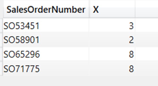
- As a result for the first row of the MAXX iteration, the X part returns value 21, which is the OrderQuantity of all the orders combined. This happens for every row of the MAXX iteration, and for every row, the X part returns the same, total OrderQuantity.

After the X iteration finishes, the MAX simply takes the MAX of the X column, which is 21. Now let’s check what happens in the correct version of the calculation.
With Context Transition
TopQTYCorrect =
MAXX(
    VALUES( FactSales[SalesOrderNumber] ),
    CALCULATE(
        SUM( FactSales[OrderQuantity] )
    )
)
The calculation is the same as the wrong one, except for the CALCULATE part.
- The 1st part of the calculation is the same, adding the virtual VALUES table with a column consisting of order numbers.
- The difference is in the X part of the MAXX function.
Prior to calculation, there is only one filter coming from the filter context, which is DimCustomer[City] =”Albany”. The X iteration starts for the first row in the table (SO53451). For the first row, it needs to perform the X calculation, which has CALCULATE function wrapped around the SUM part. When used in a row context, CALCULATE performs one extremely powerful feature called row 2 filter context transformation.
This means that every value from the current row of the iteration is transformed to a filter, which automatically travels through the model and filters it based on the conditions of that particular row. For the first row to the iteration that means that the value SO53451becomes a filter for the FactSales[SalesOrderNumber] column, and is added to the original filter context. The evaluation context for the first row of the iteration now consists of 2 filters:
DimCustomer[City] =”Albany” FactSales[SalesOrderNumber]=” SO53451”
The FactSales table in the first iteration of X looks like this:

After the CALCULATE performed its context transition, the required argument of the CALCULATE function is evaluated (SUM( FactSales[OrderQuantity] )), which returns value 3 for the first row of iteration.
The same transformation happens for every other row of the iteration, and we get correct X values for different sales orders.
After the X iteration finishes, the MAX takes the MAX of the X column, which is now a correct quantity of 8.
Referencing Measures
If we observe the wrong calculation in our previous example, we can see that as an iteration it is using the calculation SUM(FactSales[OrderQuantity]).
TopQTYWrong =
MAXX(
    VALUES( FactSales[SalesOrderNumber] ),
    SUM( FactSales[OrderQuantity] )
)
If we replace the SUM(FactSales[OrderQuantity]) function with a Measure [TotalQTY], The calculation starts to show correct figures.
TopQTYWrong = MAXX(VALUES(FactSales[SalesOrderNumber]),SUM(FactSales[OrderQuantity]))
TopQTY_Measure = MAXX(VALUES(FactSales[SalesOrderNumber]),[TotalQTY])
TotalQTY = SUM(FactSales[OrderQuantity])

The reason why referencing a measure returns the correct result is the fact that whenever you reference a Measure in other calculations, it always comes encapsulated in CALCULATE. The [TopQTY_Measure] could be read as follows:
TopQTY_Measure = MAXX(VALUES(FactSales[SalesOrderNumber]),CALCULATE([TotalQTY]))
CALCULATE will force the context transition and therefore the measure will return the correct figures.
Returning the Order Number
One thing is to return the quantity of the best order, but what if we need to return the exact order number/s of the best performing order? In that case, we need to start writing a bit more complex DAX code.
In the following example we will start combining multiple DAX concepts to provide the correct answer.
![]()
To produce the TopQTYNamemeasure we used the following DAX code:
TopQTYName =
CONCATENATEX(
    TOPN(
        1,
        ADDCOLUMNS(
            VALUES( FactSales[SalesOrderNumber] ),
            "TotalQTY", CALCULATE( SUM( FactSales[OrderQuantity] ) )
        ),
        [TotalQTY], DESC
    ),
    FactSales[SalesOrderNumber],
    "; "
)
We will explain the formula through its order of evaluation referencing row numbers in sequence. We will focus only on the cell in a visual having “Albany” filter.
Evaluation Order
Row 6 - VALUES function creates a virtual table of a single column which holds all SalesOrderNumbers of the Albany city. We can represent this table with DAX studio:
![]()
Rows 5 & 7 - ADDCOLUMNS function adds a virtual column “TotalQTY” to VALUES table. For each row of the VALUES table, we perform CALCULATE( SUM( FactSales[OrderQuantity] ) calculation that does context transition and sums quantity on the SalesOrderNumbergranularity.
![]()
Row 3 - TOPN function accepts that virtual table and then returns the top 1 row from it based on the TotalQTY virtual column.
![]()
Row 2 - CONCATENATEX takes the result of the TOPN function, then iterates through it and concatenates all SalesOrderNumbers with the highest TotalQTY. Under the “Albany” original filter, there are 2 SalesOrders with the same QTY, and they are both being concatenated and shown on the visual.
SUMMARIZE with Context Transition
If we need to make an iteration over a virtual table that consists of more columns and which needs to accept filter context, the best way would be to use SUMMARIZE.
With SUMMARIZE you can create virtual tables containing multiple columns, then iterate through them while performing context transitions.
Comments
Leave a comment
0