


Relationships are like bridges between our tables. Without them, our model would consist of isolated “islands” of data, having no direct relationships with each other. Relationships are one of the most important building blocks of the data model. You won’t define them often. Most of the time you will set relationships the moment you import your tables, and rarely you will need to introduce additional relationships into a model. But that doesn’t mean you don’t have to have a good understanding of them. They influence every measure you create in the model, and every filter you apply to a visual. That’s why you must understand them thoroughly and use them with care.
Relationship Types
There are 3 types of relationships in the Power BI data model. Each of them plays a different role in how filters travel throughout the data model and influence the result of measures.
One2Many (Power BI notation 1-* )
Already explained in the previous chapter, they form a relationship between Dimension, which has a column of unique key values, and a fact table with the foreign key consisting of the same values repeated more than once.
When forming a 1-* relationship, in a column acting as a primary key, must be no blank values. A blank value (blank row) is reserved for each primary key column to handle missing values (missing keys) coming from the foreign key column.
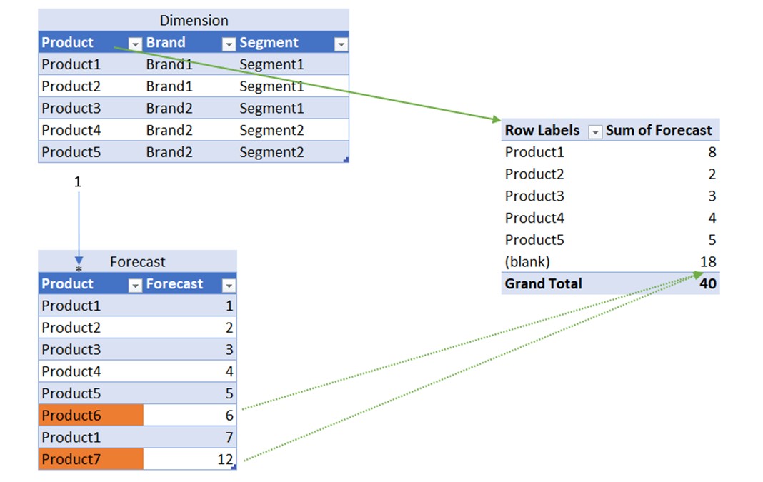
In the picture above, we have a simple data model with 2 tables (Dimension and Forecast). We created a 1-* relationship based on the product column. We plotted Dimension[Product] column in a visual (green arrow). We added [Sum Of Forecast] measure into the values field of the visual. We immediately receive a “(blank)” product label in a visual, in which all foreign keys without corresponding primary key coming from Dimension are grouped. In our case those are rows from the Forecast table with foreign keys “Product6” and “Product7”. Their sum (green dotted arrow) is plotted in the (blank) label of the visual. For the model to be able to produce a such result, it needs to add a blank value to the primary key column, which then acts as a container for all non-matched foreign keys.
One2One (Power BI notation 1-1 )
Rarely used since tables connected through this relationship are, in most situations, transformed into a single table. It’s a relationship in which both key columns consist of unique values.
Many2Many (Power BI notation *-*)
Relationship in which neither key column must have unique values. This type of relationship is extremely dangerous in case of using it in the wrong places or without a clear understanding of its possible implications for your calculations.
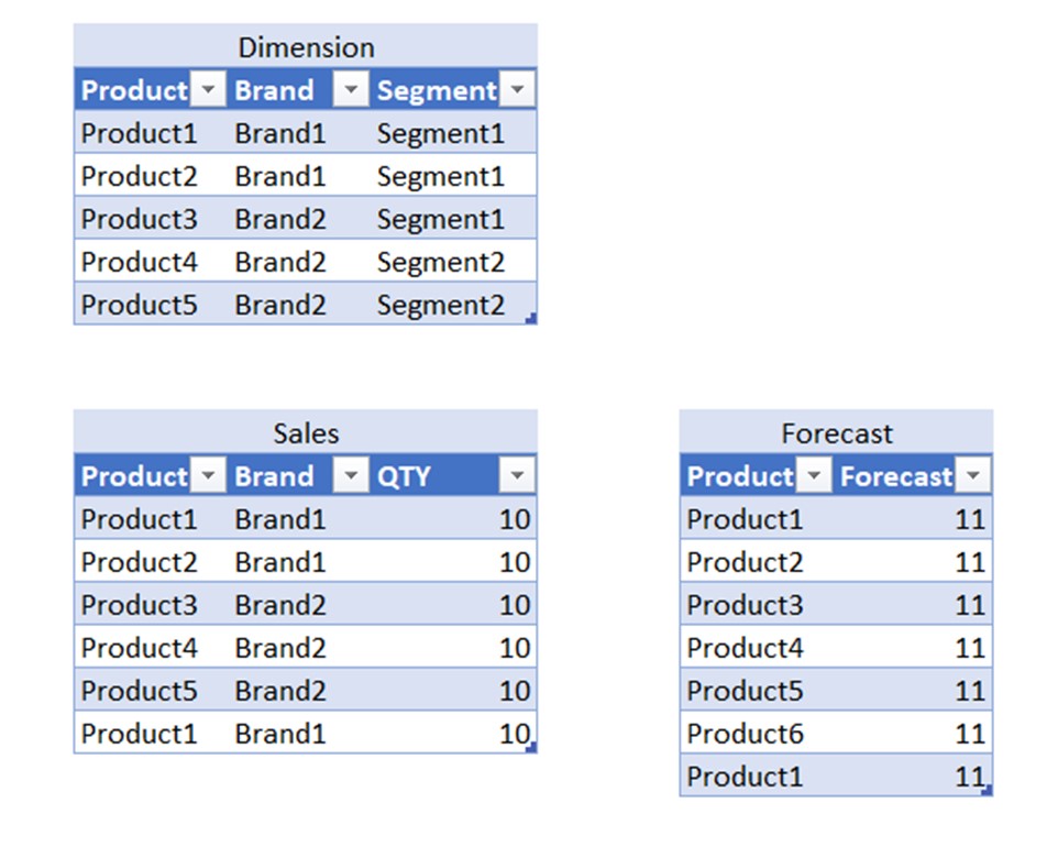
To understand how M2M operates and why it is a dangerous relationship, let’s check the following example. We will try to keep it as simple as possible. These are the tables we will use in our example. We have one dimension table and 2 fact ones.
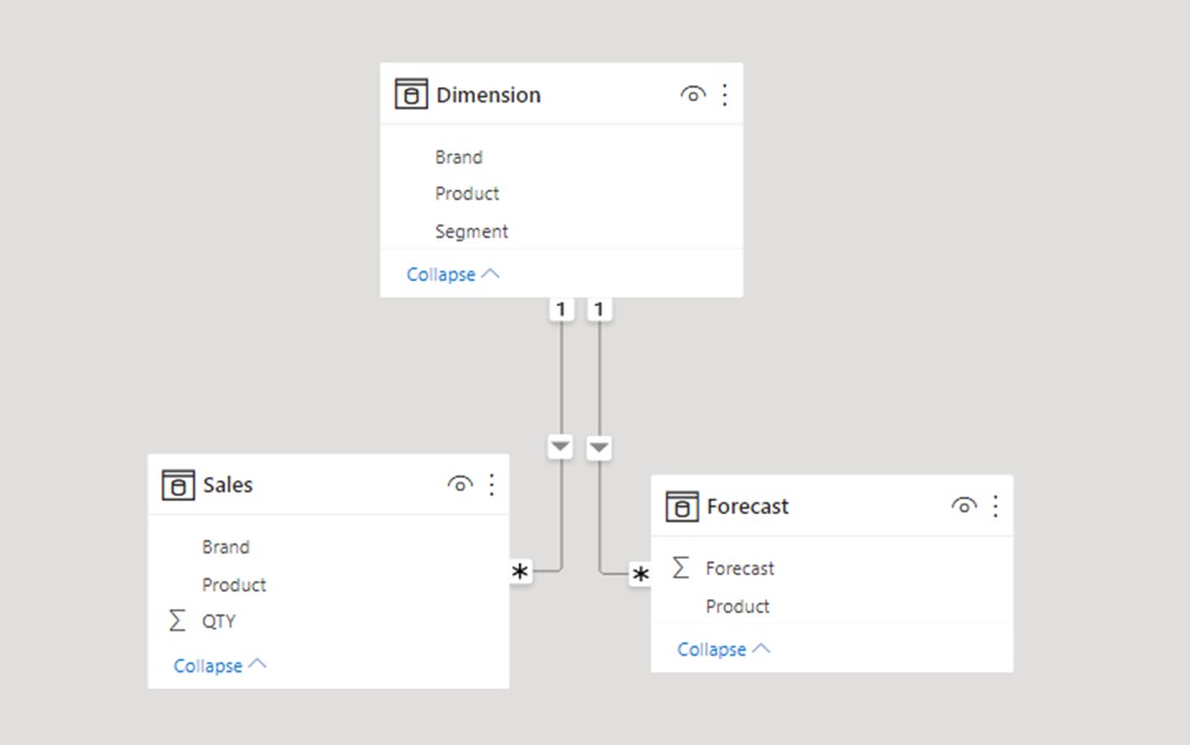
First, let’s connect both fact tables with dimension through 1-* relationship and let’s plot the values on the visual (using product columns as keys).
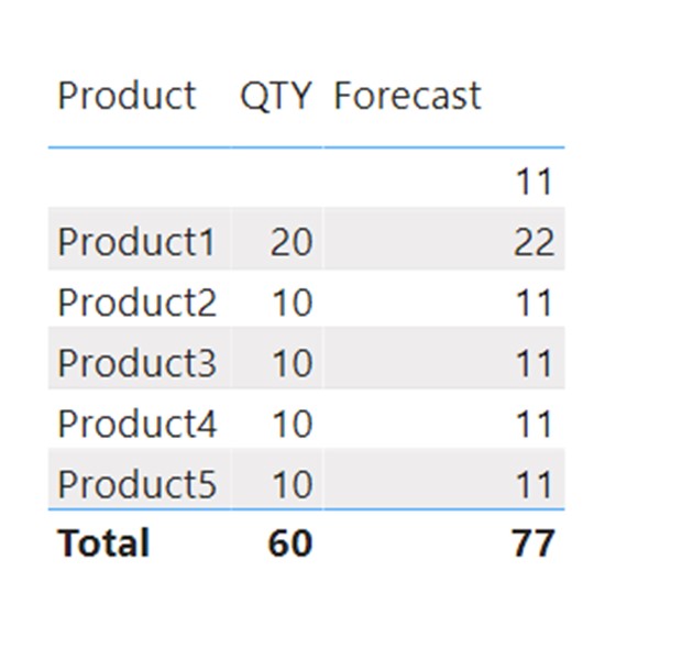
When we put the product from the dimension into a visual and add QTY and Forecast calculations to the visual, we can clearly see that there is a missing value in the dimension (product 6), and we receive a blank row in a visual which contains the forecast value for the non-matched key. There is a clear indicator that there is a missing key in the dimension, and we can act accordingly.
Now let’s connect Sales and Forecast tables directly through the M2M relationship. We will use Product as a key column in both tables and plot product from the Sales table as a filter.
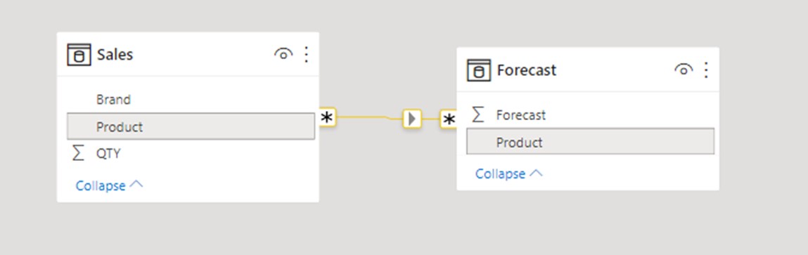
We receive a different, and quite dangerous result.
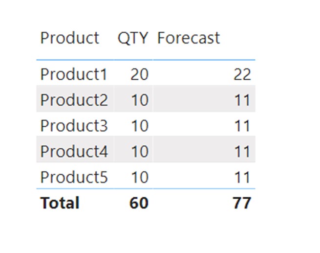
Even though there is no Product6 in the Sales table, when we plot Forecast, we do not receive a blank row indicating that there are missing keys in a relationship. We can only assume that if we check the difference between figures in the visual compared to the total value of the forecast. Only then we would notice that 11 Forecast QTY is missing in the visual. This could be noticed on the small dataset or visual with few filters and simple calculations, but in more complex scenarios it would be impossible. We would have missing values in visual without even noticing they are missing. When using M2M you will never receive a blank row for handling the missing keys in a relationship.
Now let’s check the second possible mistake we could make with the wrong M2M relationship. This time we will connect Dimension with Sales, but we will use Brand as a key column:
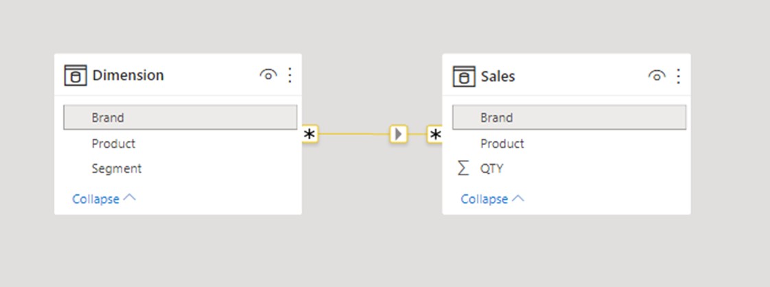
We will plot the Segment column from the Dimension table onto a visual, and once again, the values in the visual make little sense.
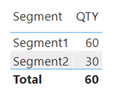
We can clearly see that the sum of segments is larger than the sum of the total. This can’t be correct, so what is happening with the relationship that is causing this strange behavior?
The picture below should shed some light on it:
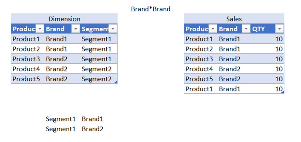
We will focus on Segment1, which has a value of 60. We can see that Segment1 has products that fall under brands “Brand1” and “Brand2”. Our relationship is formed based on brand columns, so for Segment1, both Brand1 and Brand2 filters will travel through the relationship and filter the sales table. Since the sales table consists of only Brand1 and Brand2 in the Brand column, the value returned in the visual is the total sum of all brands.
This is a simple example, and it might seem you would never fall into this mistake, but when using M2M, if you have any kind of filters that overlap (e.g. same brands can be under multiple segments), you are in danger of having your values multiplied and showing false results in the visual.
Disadvantages of M2M:
- Could easily lead to false calculations if used improperly
- Extremely slow in case of high cardinality columns used in the relationship
- Does not follow data modeling best practices
To conclude, you should use the M2M type of relationship only as a last resort, and only if you understand its implications for the data model.