


Measure Explanation
Measures are the most important objects in your data models. They are the ones that provide dynamic results based on different combinations of filters plotted on visuals. They are also the most complex ones since they change results with each interaction in a report. To be able to produce the correct result while we slice and dice the data, they operate under a strict set of concepts that interact in a logical way. We will cover those concepts later on, but for now, let’s get familiar with a simple explanation.
We find it most convenient to explain measures through a small table linked to a PivotTable. This makes it easier for a reader to understand them more vividly. They function the same way in our example as in huge, several gigabytes data models.
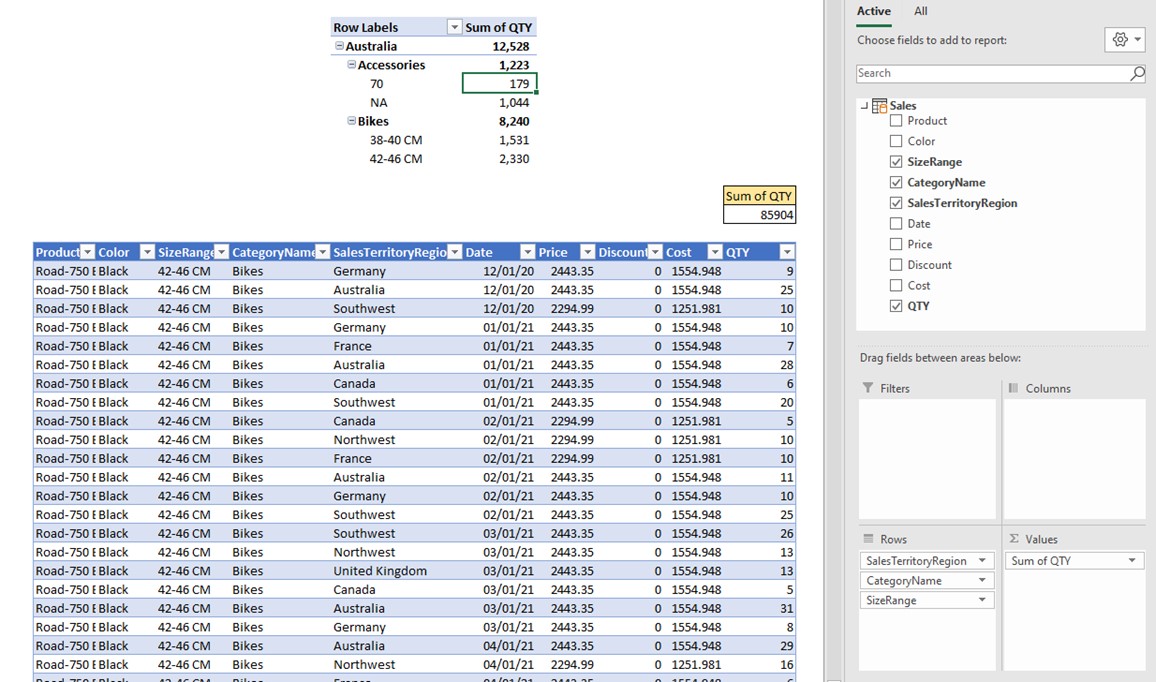
On the top of the picture above we have a regular PivotTable, and on the bottom part is a data source table called Sales. As we can see on the pane to the right of the table, we pulled SalesTerritoryRegion, CategoryName, and SizeRange columns into “Rows” field of the Pivot, and QTY column into the “Values” field.
We will first explain how the PivotTable returned number 179 under the filters Australia-Accessories-70.
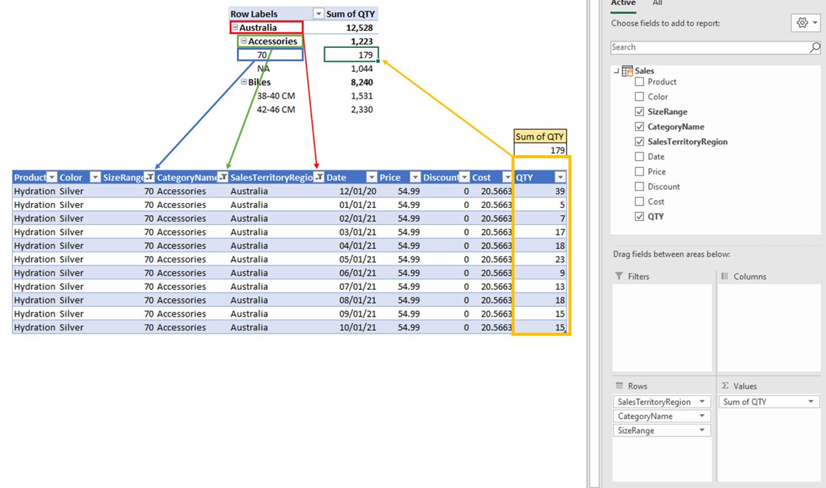
Every time you debug a result of a visual (in our case PivotTable), you should focus on a single point/cell of the visual.
The 1st step of calculating any result in a visual is to check which filters are influencing the visual in a selected point.
For the selected point (cell) which returns the number 179, these are the filters influencing the calculation:
- Sales[SalesCategoryFilters]= “Australia”
- Sales[CategoryName]=”Accessories”
- Sales[SizeRange]=”70”
Those conditions are filtering the data source table and only rows that fall under all 3 conditions survive. The filters are represented with blue, green, and red arrows. The only arrow left is the yellow one. The yellow arrow represents the calculation (value) which is returned to the visual once the filtering part has finished. The order of evaluation for each cell in the visual is the following:
- Filtering part
- Calculation (Measure)
In our simple example, the calculation is the Sum Of QTY, which represent the DAX calculation [Sum Of QTY] = SUM(Sales[QTY]). [Sum of QTY] calculation sums the values from the column Sales[QTY] of the Sales table respecting the rows which survived the filtering part.
Why do we need the SUM Function in a calculation?
Calculations operate on rows of the table which survived the filter conditions coming from visuals. Most of the time there will be more than one row that survived the filtering part. If we weren’t to use aggregation functions (SUM, MIN, MAX, COUNT, DISTINCTCOUNT, AVERAGE, etc.), the calculation would try to return non aggregated values (multiple rows in a table/column) in a single point in a visual. This is not possible in DAX and you will get an error stating that you tried to supply multiple rows where a single value was expected.

The filtering part of the calculation evaluation is determined by the values of the columns plotted in the rows field of the PivotTable visual. DAX calculation is the same for each cell of the visual, but since different filters are applied prior to the calculation, so does the result change.
The same rules apply for subtotals and grand total.
How Totals Are Calculated?
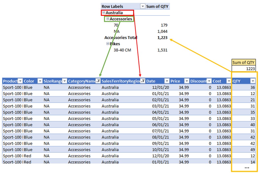
Accessories Total is not calculated by the visual sum of SizeRange “70” and “NA”. Instead, it is calculated in the same fashion of filtering the data source table. But for the Accessories total point, only 2 filters are applied to the source table prior to the calculation. Those are:
- Sales[SalesCategoryFilters]= “Australia”
- Sales[CategoryName]=”Accessories”
After these filters are applied to the source, the calculation kicks in and sums the QTY of the rows which survived the filtering part.
The calculation part always starts after the initial filters are applied to the point in a visual. The calculation can be a simple one (such as SUM(ColumnName)), but also a complex one, involving many different columns from table/s. You can pretty much write DAX code of any level of complexity to return the needed result for the selected point of the visual and even interfere with the original filters, as we will explain in the CALCULATE chapter.
Now as for the terminology, the filtering part of any point in a visual that is occurring prior to the calculation is called the original filter context. The calculation that starts after the original filter context has been formed is called Measure. Since the original filter context is always different for each point in a visual, so does the measure return different results.
The hardest part of writing an efficient DAX code is understaning how to utilize the original filter context! Seasoned DAX coders never write code that works against filter context, but alongide it. It take a lot of practice and training to understand well which parts of formula logic should be written with DAX and which should be left for the filter context to handle.
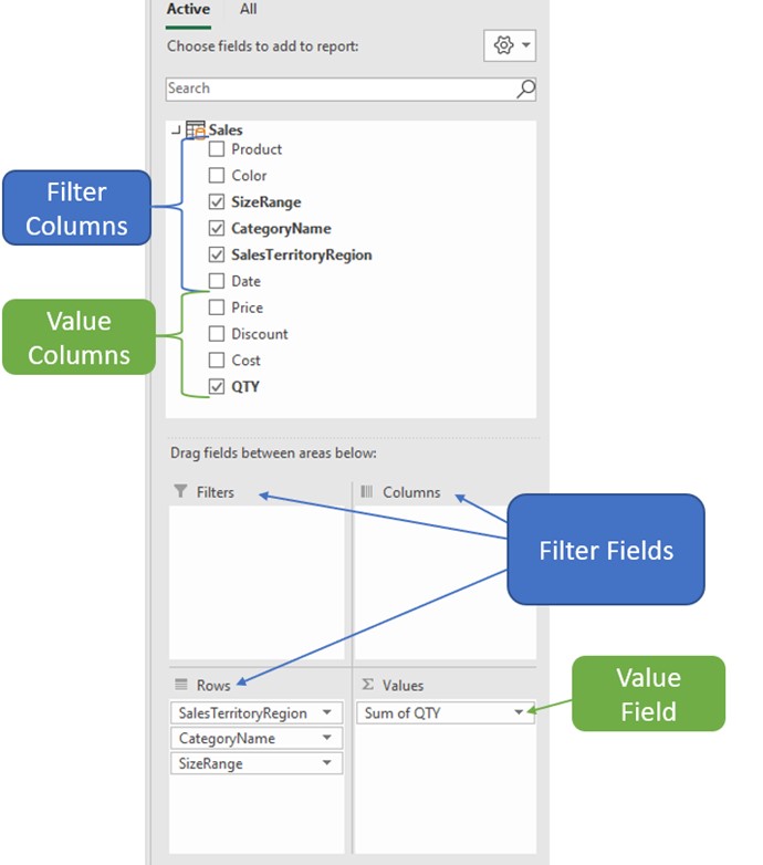
Types of Fields in Visuals
Each visual in Power BI (or PivotTable in Excel) accepts only 2 types of fields. This is true for any other type of visual no matter how many fields it accepts.
Filter fields:
Fields that accept a distinct combination of values from columns plotted on the visual. In our example, Pivot fields “Filters”, ”Columns”, and “Rows” are all of the same Filter fields type.
Values fields:
Fields that accept only Measures as inputs.
You might think this statement is not correct since we can drag the Columns from the table into a Values field and they will return value, even though we haven’t defined a Measure. But in fact, when we drag Column into a Values field of the visual, we create an implicit Measure. That is why we always receive “Sum of” or “Count of” prefix before the name of the column plotted in the Values field of the PivotTable. In our example, since we dragged the QTY column to the Values field, the model internally created an implicit measure named [Sum of QTY].
We should never use this type of measure, but always create an explicit one in the model. Why?
- Implicit measures cannot be referenced with other measures.
- Their calculations are limited to only 8 main aggregations (SUM, MIN, MAX, COUNT, DISTINCT, ST DEV, VAR, AND MEDIAN)
- They are local to each visual
Which Columns to Use in Measures
Now let’s explain which columns in the table are most suitable for filter fields, and which to form Measures. Just as fields in a visual, tables also contain 2 main types of columns. Those are Filter and Value columns.
The difference?
Filter columns are mostly used in a visual to form the visual representation of the data (the original filter context), in which the calculation should execute. Value columns are mostly used to return results.
How to make a distinction?
Filter columns are the ones you will mostly plot in filter fields of the visual.
Values columns are mostly used to create Measures that we can plot only in Values fields of the visual.
In our Sales table, the best split of the column types would be the following:
- Filter columns:
- Product
- Color
- SizeRange
- CategoryName
- SalesTerritoryRegion
- Date
- Value columns:
- Price
- Discount
- Cost
- QTY
Filter columns are used quite often in Measures, but mostly in intermediate steps (unless we need to count the number of distinct values of the column). Value columns are almost never used in Filter fields of the visual, especially if not grouped.
Measure features
Measures are built for speed, meaning they consume mostly CPU power and can produce fast results no matter how much we filter the data (unless we write poor DAX or overuse filters).
Their results are evaluated on each interaction with the visuals (slicing, filtering, cross-filtering). If you have 20 visuals on a report page, on each interaction with the data (eq. selecting a slicer), you will send at least 20 queries to the underlying model. Those queries are grouped by filters coming from columns plotted on visuals.
Other important Measure features:
- Measures are always under the influence of the canvas’s original filter context (columns plotted on visuals);
- Filter context is formed with the use of filtering columns dragged to the visual from your data model;
- You should always use explicit measures, and avoid using implicit measures;
- Measures can return only a single value in a single point of the visual, therefore you always need to aggregate rows of the columns/tables you use in a Measure. (SUM, MIN, COUNT, etc.);
- Measures use both filtering and value columns in producing a result
- Filtering columns are mainly used as intermediate building blocks of the code (e.g. iteration over the list of values, arguments to CALCULATE). They can also be used to return count or distinct count of selected column/s as result.
- Value columns are used both in intermediate steps and to return the final result.