


This segmentation somewhat differs from the generally accepted one, but we find it most suitable to explain different types of CALCULATE filter arguments. In case you find any part of our explanation not precise enough, feel free to comment.
CALCULATE accepts 3 types of filter arguments. Those are model modifiers, model filter removers, and tables of supplied new values. It’s important to understand the distinction between the 3 of them because they play separate roles in the CALCULATE evaluation order.
Model Modifiers
Model modifiers change the semantics of the data model for the specified measure. Those changes include activating non-active relationships or setting cross filter directions.
CROSSFILTER and USERELATIONSHIP functions are the most commonly used model modifiers functions.
Model Filter Removers
Functions mostly used to ignore column/table filters are REMOVEFILTERS and ALL. ALL function can also be used as a supplied table function (3rd type of CALCULATE filter argument) if not used as a top level filter function.
- If ALL is used as ALL(ColumnName) then it acts as a filter remover and has the same effect as REMOVEFILTERS(ColumnName) function.
- If ALL is used as FILTER(ALL(ColumnName),true) then it acts as a model filter that can produce a different result in certain situations.
When used as filter remover, both ALL and REMOVEFILTERS functions perform in the same manner, meaning they remove columns used as arguments from the filter context.
ALL with column argument vs ALL with table argument
ALL function behaves differently when you supply a whole table as an input as opposed to a column. Let’s explain this with the following example.
AllFactTable = CALCULATE([SalesAmount],ALL(FactSales))
AllCategoryName = CALCULATE([SalesAmount],ALL(DimProduct[CategoryName]))
In the visual below, DimProduct[CategoryName] and DimCustomer[Country] columns are plotted from DimProduct and DimCustomer tables that are connected to the FactSales table through a 1-* relationship.
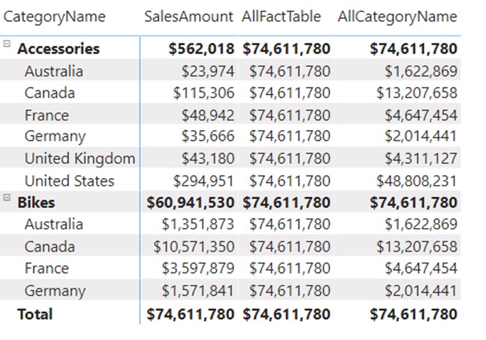
AllFactTable measure: When we use table reference as a filter argument, we are ignoring all filters coming from that table, but we also ignore all filters coming from other tables linked to that table through a 1-* relationship. This feature is called expanded tables (covered here).
In the picture above we can see that, even though we haven’t removed any column from the DimProduct or DimCustomer, we still ignore all columns coming from these tables, including DimProduct[CategoryName] and DimCustomer[Country].
AllCategoryName measure: This measure is using column reference in the filter argument, meaning it’s not working with the expanded tables version, but instead it ignores only the specified DimProduct[CategoryName] column. If we focus on the Accessories – Australia cell in the visual, we can see that it produces a different result compared to the total Accessories. Which number does it return? Since we only ignored DimProduct[CategoryName] column, the Country filter is still active for the calculation. This cell returns the total SalesAmount of all sales coming from Australia. And if we observe the values for Bikes, we can see that the figures repeat.
This way we can ignore specific columns/tables from active filters before we run CALCULATE expression.
Table of new values
As opposed to ignoring specific column/table filters, this type of filter argument supplies a set of new active values for columns used in the CALCULATE filter argument.
You can supply either single-column or multi-column combinations of filters that are different than the ones applied with the original filter context. Let’s explain this feature with the calculation below.
Blue or Accessories Summarize =
CALCULATE(
    [SalesAmount],
    FILTER(
        SUMMARIZE(
            Sales,
            Sales[Color],
            Sales[CategoryName]
        ),
        Sales[Color] = "Blue"
            || Sales[CategoryName] = "Accessories"
    )
)
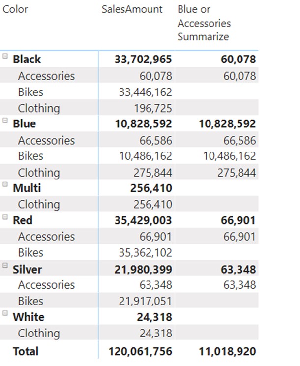
This time, instead of ignoring columns prior to calculation, we provide a list (or table) with the values that must further filter the original filter context before the calculation starts. In the example above, we use SUMMARIZE function to create an OR argument for the SalesAmount calculation. The summarized virtual table looks like this:
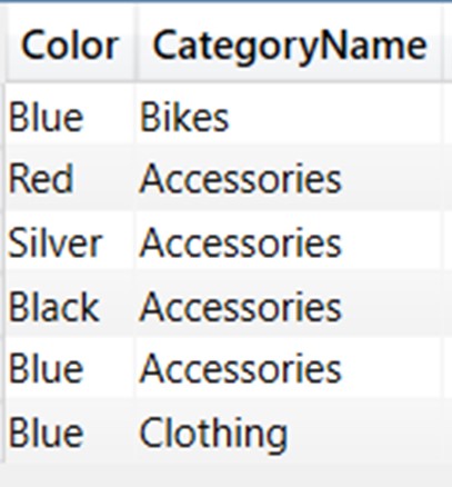
Those values now become filters that further filter the Sales table, resulting in the values seen in the visual above.
You will use SUMMARIZE function quite often when you will need to provide a modified lists of values that will futher filter the original filter context. SUMMARIZE is also often used to create a table over which you want to create row 2 filter context transition. This topic will be covered in the following article.
Difference Between Modifiers and Filter/Remove Arguments
Besides the obvious differences in their use cases, it is important to acknowledge that modifiers always have precedence before table filter arguments. This makes sense because you always want to modify the data model (e.g. activate a specific relationship using the USERELATIONSHIP function) before applying any other data model filter argument.